睿智的目标检测40——Keras搭建Retinaface人脸检测与关键点定位平台
睿智的目标检测40——Keras搭建Retinaface人脸检测与关键点定位平台
- 学习前言
- 什么是Retinaface人脸检测算法
- 源码下载
- Retinaface实现思路
- 一、预测部分
- 1、主干网络介绍
- 2、FPN特征金字塔
- 3、SSH进一步加强特征提取
- 4、从特征获取预测结果
- 5、预测结果的解码
- 6、在原图上进行绘制
- 二、训练部分
- 1、真实框的处理
- 2、利用处理完的真实框与对应图片的预测结果计算loss
- 训练自己的Retinaface模型
学习前言
一起来看看Retinaface的keras实现吧。
什么是Retinaface人脸检测算法
Retinaface是来自insightFace的又一力作,基于one-stage的人脸检测网络。
同时开源了代码与数据集,在widerface上有非常好的表现。
源码下载
https://github.com/bubbliiiing/retinaface-keras
喜欢的可以点个star噢。
Retinaface实现思路
一、预测部分
1、主干网络介绍
Retinaface在实际训练的时候使用两种网络作为主干特征提取网络。分别是MobilenetV1-0.25和Resnet。
使用Resnet可以实现更高的精度,使用MobilenetV1-0.25可以在CPU上实现实时检测。
本文以MobilenetV1-0.25进行展示。
MobileNet模型是Google针对手机等嵌入式设备提出的一种轻量级的深层神经网络,其使用的核心思想便是depthwise separable convolution。
对于一个卷积点而言:
假设有一个3×3大小的卷积层,其输入通道为16、输出通道为32。具体为,32个3×3大小的卷积核会遍历16个通道中的每个数据,最后可得到所需的32个输出通道,所需参数为16×32×3×3=4608个。
应用深度可分离卷积,用16个3×3大小的卷积核分别遍历16通道的数据,得到了16个特征图谱。在融合操作之前,接着用32个1×1大小的卷积核遍历这16个特征图谱,所需参数为16×3×3+16×32×1×1=656个。
可以看出来depthwise separable convolution可以减少模型的参数。
如下这张图就是depthwise separable convolution的结构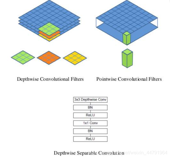
在建立模型的时候,可以使用Keras中的DepthwiseConv2D层实现深度可分离卷积,然后再利用1x1卷积调整channels数。
通俗地理解就是3x3的卷积核厚度只有一层,然后在输入张量上一层一层地滑动,每一次卷积完生成一个输出通道,当卷积完成后,在利用1x1的卷积调整厚度。
如下就是MobileNet的结构,其中Conv dw就是分层卷积,在其之后都会接一个1x1的卷积进行通道处理,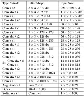
上图所示是的mobilenetV1-1的结构,本文所用的mobilenetV1-0.25是mobilenetV1-1通道数压缩为原来1/4的网络。
import warningsimport numpy as npfrom keras.models import Modelfrom keras.layers import DepthwiseConv2D,Input,Activation,Dropout,Reshape,BatchNormalization,GlobalAveragePooling2D,GlobalMaxPooling2D,Conv2Dfrom keras import backend as Kdef _conv_block(inputs, filters, kernel=(3, 3), strides=(1, 1)):x = Conv2D(filters, kernel,padding='same',use_bias=False,strides=strides,name='conv1')(inputs)x = BatchNormalization(name='conv1_bn')(x)return Activation(relu6, name='conv1_relu')(x)def _depthwise_conv_block(inputs, pointwise_conv_filters,depth_multiplier=1, strides=(1, 1), block_id=1):x = DepthwiseConv2D((3, 3),padding='same',depth_multiplier=depth_multiplier,strides=strides,use_bias=False,name='conv_dw_%d' % block_id)(inputs)x = BatchNormalization(name='conv_dw_%d_bn' % block_id)(x)x = Activation(relu6, name='conv_dw_%d_relu' % block_id)(x)x = Conv2D(pointwise_conv_filters, (1, 1),padding='same',use_bias=False,strides=(1, 1),name='conv_pw_%d' % block_id)(x)x = BatchNormalization(name='conv_pw_%d_bn' % block_id)(x)return Activation(relu6, name='conv_pw_%d_relu' % block_id)(x)def relu6(x):return K.relu(x, max_value=6)def MobileNet(img_input, depth_multiplier=1):x = _conv_block(img_input, 8, strides=(2, 2))x = _depthwise_conv_block(x, 16, depth_multiplier, block_id=1)x = _depthwise_conv_block(x, 32, depth_multiplier, strides=(2, 2), block_id=2)x = _depthwise_conv_block(x, 32, depth_multiplier, block_id=3)x = _depthwise_conv_block(x, 64, depth_multiplier, strides=(2, 2), block_id=4)x = _depthwise_conv_block(x, 64, depth_multiplier, block_id=5)feat1 = xx = _depthwise_conv_block(x, 128, depth_multiplier, strides=(2, 2), block_id=6)x = _depthwise_conv_block(x, 128, depth_multiplier, block_id=7)x = _depthwise_conv_block(x, 128, depth_multiplier, block_id=8)x = _depthwise_conv_block(x, 128, depth_multiplier, block_id=9)x = _depthwise_conv_block(x, 128, depth_multiplier, block_id=10)x = _depthwise_conv_block(x, 128, depth_multiplier, block_id=11)feat2 = xx = _depthwise_conv_block(x, 256, depth_multiplier, strides=(2, 2), block_id=12)x = _depthwise_conv_block(x, 256, depth_multiplier, block_id=13)feat3 = xreturn feat1, feat2, feat3
2、FPN特征金字塔

与Retinanet类似的是,Retinaface使用了FPN的结构,对Mobilenet最后三个shape的有效特征层进行FPN结构的构建。
构建方式很简单,首先利用1x1卷积对三个有效特征层进行通道数的调整。调整后利用Upsample和Add进行上采样的特征融合。
实现代码为:
def RetinaFace(cfg, backbone="mobilenet"):inputs = Input(shape=(None, None, 3))if backbone == "mobilenet":C3, C4, C5 = MobileNet(inputs)elif backbone == "resnet50":C3, C4, C5 = ResNet50(inputs)else:raise ValueError('Unsupported backbone - `{}`, Use mobilenet, resnet50.'.format(backbone))leaky = 0if (cfg['out_channel'] <= 64):leaky = 0.1P3 = Conv2D_BN_Leaky(cfg['out_channel'], kernel_size=1, strides=1, padding='same', name='C3_reduced', leaky=leaky)(C3)P4 = Conv2D_BN_Leaky(cfg['out_channel'], kernel_size=1, strides=1, padding='same', name='C4_reduced', leaky=leaky)(C4)P5 = Conv2D_BN_Leaky(cfg['out_channel'], kernel_size=1, strides=1, padding='same', name='C5_reduced', leaky=leaky)(C5)P5_upsampled = UpsampleLike(name='P5_upsampled')([P5, P4])P4 = Add(name='P4_merged')([P5_upsampled, P4])P4 = Conv2D_BN_Leaky(cfg['out_channel'], kernel_size=3, strides=1, padding='same', name='Conv_P4_merged', leaky=leaky)(P4)P4_upsampled = UpsampleLike(name='P4_upsampled')([P4, P3])P3 = Add(name='P3_merged')([P4_upsampled, P3])P3 = Conv2D_BN_Leaky(cfg['out_channel'], kernel_size=3, strides=1, padding='same', name='Conv_P3_merged', leaky=leaky)(P3)
3、SSH进一步加强特征提取
通过第二部分的运算,我们获得了P3、P4、P5三个有效特征层。
Retinaface为了进一步加强特征提取,使用了SSH模块加强感受野。
SSH的结构如如下所示:
SSH的思想非常简单,使用了三个并行结构,利用3x3卷积的堆叠代替5x5与7x7卷积的效果:左边的是3x3卷积,中间利用两次3x3卷积代替5x5卷积,右边利用三次3x3卷积代替7x7卷积。
这个思想在Inception里面有使用。
SSH实现代码为:
def SSH(inputs, out_channel, leaky=0.1):conv3X3 = Conv2D_BN(out_channel//2, kernel_size=3, strides=1, padding='same')(inputs)conv5X5_1 = Conv2D_BN_Leaky(out_channel//4, kernel_size=3, strides=1, padding='same', leaky=leaky)(inputs)conv5X5 = Conv2D_BN(out_channel//4, kernel_size=3, strides=1, padding='same')(conv5X5_1)conv7X7_2 = Conv2D_BN_Leaky(out_channel//4, kernel_size=3, strides=1, padding='same', leaky=leaky)(conv5X5_1)conv7X7 = Conv2D_BN(out_channel//4, kernel_size=3, strides=1, padding='same')(conv7X7_2)out = Concatenate(axis=-1)([conv3X3, conv5X5, conv7X7])out = Activation("relu")(out)return out
Retinaface会将我们获得的P3、P4、P5三个有效特征层。都施加上SSH结构。
实现代码为:
def RetinaFace(cfg, backbone="mobilenet"):inputs = Input(shape=(None, None, 3))if backbone == "mobilenet":C3, C4, C5 = MobileNet(inputs)elif backbone == "resnet50":C3, C4, C5 = ResNet50(inputs)else:raise ValueError('Unsupported backbone - `{}`, Use mobilenet, resnet50.'.format(backbone))leaky = 0if (cfg['out_channel'] <= 64):leaky = 0.1P3 = Conv2D_BN_Leaky(cfg['out_channel'], kernel_size=1, strides=1, padding='same', name='C3_reduced', leaky=leaky)(C3)P4 = Conv2D_BN_Leaky(cfg['out_channel'], kernel_size=1, strides=1, padding='same', name='C4_reduced', leaky=leaky)(C4)P5 = Conv2D_BN_Leaky(cfg['out_channel'], kernel_size=1, strides=1, padding='same', name='C5_reduced', leaky=leaky)(C5)P5_upsampled = UpsampleLike(name='P5_upsampled')([P5, P4])P4 = Add(name='P4_merged')([P5_upsampled, P4])P4 = Conv2D_BN_Leaky(cfg['out_channel'], kernel_size=3, strides=1, padding='same', name='Conv_P4_merged', leaky=leaky)(P4)P4_upsampled = UpsampleLike(name='P4_upsampled')([P4, P3])P3 = Add(name='P3_merged')([P4_upsampled, P3])P3 = Conv2D_BN_Leaky(cfg['out_channel'], kernel_size=3, strides=1, padding='same', name='Conv_P3_merged', leaky=leaky)(P3)SSH1 = SSH(P3, cfg['out_channel'], leaky=leaky)SSH2 = SSH(P4, cfg['out_channel'], leaky=leaky)SSH3 = SSH(P5, cfg['out_channel'], leaky=leaky)SSH_all = [SSH1,SSH2,SSH3]
4、从特征获取预测结果
通过第三步,我们已经可以获得SSH1,SSH2,SHH3三个有效特征层了。在获得这三个有效特征层后,我们需要通过这三个有效特征层获得预测结果。
Retinaface的预测结果分为三个,分别是分类预测结果,框的回归预测结果和人脸关键点的回归预测结果。
1、分类预测结果用于判断先验框内部是否包含物体,原版的Retinaface使用的是softmax进行判断。此时我们可以利用一个1x1的卷积,将SSH的通道数调整成num_anchors x 2,用于代表每个先验框内部包含人脸的概率。
2、框的回归预测结果用于对先验框进行调整获得预测框,我们需要用四个参数对先验框进行调整。此时我们可以利用一个1x1的卷积,将SSH的通道数调整成num_anchors x 4,用于代表每个先验框的调整参数。
3、人脸关键点的回归预测结果用于对先验框进行调整获得人脸关键点,每一个人脸关键点需要两个调整参数,一共有五个人脸关键点。此时我们可以利用一个1x1的卷积,将SSH的通道数调整成num_anchors x 10(num_anchors x 5 x 2),用于代表每个先验框的每个人脸关键点的调整。
实现代码为:
def ClassHead(inputs, num_anchors=2):outputs = Conv2D(num_anchors*2, kernel_size=1, strides=1)(inputs)return Activation("softmax")(Reshape([-1,2])(outputs))def BboxHead(inputs, num_anchors=2):outputs = Conv2D(num_anchors*4, kernel_size=1, strides=1)(inputs)return Reshape([-1,4])(outputs)def LandmarkHead(inputs, num_anchors=2):outputs = Conv2D(num_anchors*10, kernel_size=1, strides=1)(inputs)return Reshape([-1,10])(outputs)def RetinaFace(cfg, backbone="mobilenet"):inputs = Input(shape=(None, None, 3))if backbone == "mobilenet":C3, C4, C5 = MobileNet(inputs)elif backbone == "resnet50":C3, C4, C5 = ResNet50(inputs)else:raise ValueError('Unsupported backbone - `{}`, Use mobilenet, resnet50.'.format(backbone))leaky = 0if (cfg['out_channel'] <= 64):leaky = 0.1P3 = Conv2D_BN_Leaky(cfg['out_channel'], kernel_size=1, strides=1, padding='same', name='C3_reduced', leaky=leaky)(C3)P4 = Conv2D_BN_Leaky(cfg['out_channel'], kernel_size=1, strides=1, padding='same', name='C4_reduced', leaky=leaky)(C4)P5 = Conv2D_BN_Leaky(cfg['out_channel'], kernel_size=1, strides=1, padding='same', name='C5_reduced', leaky=leaky)(C5)P5_upsampled = UpsampleLike(name='P5_upsampled')([P5, P4])P4 = Add(name='P4_merged')([P5_upsampled, P4])P4 = Conv2D_BN_Leaky(cfg['out_channel'], kernel_size=3, strides=1, padding='same', name='Conv_P4_merged', leaky=leaky)(P4)P4_upsampled = UpsampleLike(name='P4_upsampled')([P4, P3])P3 = Add(name='P3_merged')([P4_upsampled, P3])P3 = Conv2D_BN_Leaky(cfg['out_channel'], kernel_size=3, strides=1, padding='same', name='Conv_P3_merged', leaky=leaky)(P3)SSH1 = SSH(P3, cfg['out_channel'], leaky=leaky)SSH2 = SSH(P4, cfg['out_channel'], leaky=leaky)SSH3 = SSH(P5, cfg['out_channel'], leaky=leaky)SSH_all = [SSH1,SSH2,SSH3]bbox_regressions = Concatenate(axis=1,name="bbox_reg")([BboxHead(feature) for feature in SSH_all])classifications = Concatenate(axis=1,name="cls")([ClassHead(feature) for feature in SSH_all])ldm_regressions = Concatenate(axis=1,name="ldm_reg")([LandmarkHead(feature) for feature in SSH_all])output = [bbox_regressions, classifications, ldm_regressions]model = Model(inputs=inputs, outputs=output)return model
5、预测结果的解码
通过第四步,我们可以获得三个有效特征层SSH1、SSH2、SSH3。
这三个有效特征层相当于将整幅图像划分成不同大小的网格,当我们输入进来的图像是(640, 640, 3)的时候。
SSH1的shape为(80, 80, 64);
SSH2的shape为(40, 40, 64);
SSH3的shape为(20, 20, 64)
SSH1就表示将原图像划分成80x80的网格;SSH2就表示将原图像划分成40x40的网格;SSH3就表示将原图像划分成20x20的网格,每个网格上有两个先验框,每个先验框代表图片上的一定区域。
Retinaface的预测结果用来判断先验框内部是否包含人脸,并且对包含人脸的先验框进行调整获得预测框与人脸关键点。
1、分类预测结果用于判断先验框内部是否包含物体,我们可以利用一个1x1的卷积,将SSH的通道数调整成num_anchors x 2,用于代表每个先验框内部包含人脸的概率。
2、框的回归预测结果用于对先验框进行调整获得预测框,我们需要用四个参数对先验框进行调整。此时我们可以利用一个1x1的卷积,将SSH的通道数调整成num_anchors x 4,用于代表每个先验框的调整参数。每个先验框的四个调整参数中,前两个用于对先验框的中心进行调整,后两个用于对先验框的宽高进行调整。
3、人脸关键点的回归预测结果用于对先验框进行调整获得人脸关键点,每一个人脸关键点需要两个调整参数,一共有五个人脸关键点。此时我们可以利用一个1x1的卷积,将SSH的通道数调整成num_anchors x 10(num_anchors x 5 x 2),用于代表每个先验框的每个人脸关键点的调整。每个人脸关键点的两个调整参数用于对先验框中心的x、y轴进行调整获得关键点坐标。
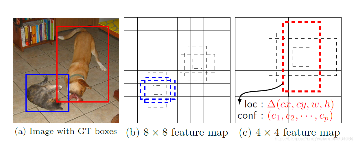
完成调整、判断之后,还需要进行非极大移植。
下图是经过非极大抑制的。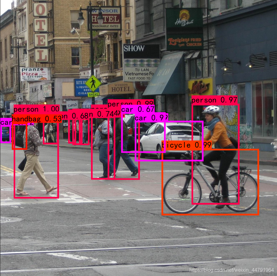
下图是未经过非极大抑制的。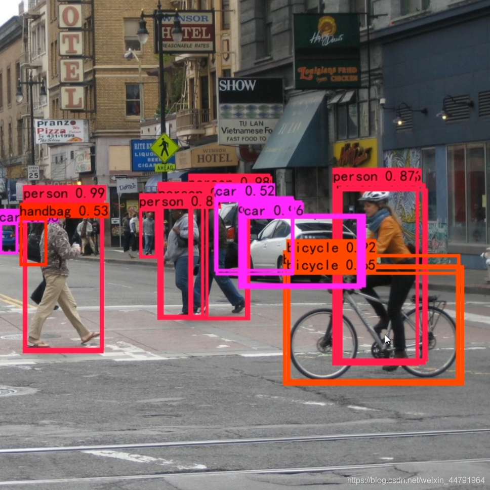
可以很明显的看出来,未经过非极大抑制的图片有许多重复的框,这些框都指向了同一个物体!
可以用一句话概括非极大抑制的功能就是:
筛选出一定区域内属于同一种类得分最大的框。
全部实现代码如下:
class BBoxUtility(object):def __init__(self, priors=None, overlap_threshold=0.35,nms_thresh=0.45):self.priors = priorsself.num_priors = 0 if priors is None else len(priors)self.overlap_threshold = overlap_thresholdself._nms_thresh = nms_threshdef decode_boxes(self, mbox_loc, mbox_ldm, mbox_priorbox):# 获得先验框的宽与高prior_width = mbox_priorbox[:, 2] - mbox_priorbox[:, 0]prior_height = mbox_priorbox[:, 3] - mbox_priorbox[:, 1]# 获得先验框的中心点prior_center_x = 0.5 * (mbox_priorbox[:, 2] + mbox_priorbox[:, 0])prior_center_y = 0.5 * (mbox_priorbox[:, 3] + mbox_priorbox[:, 1])# 真实框距离先验框中心的xy轴偏移情况decode_bbox_center_x = mbox_loc[:, 0] * prior_width * 0.1decode_bbox_center_x += prior_center_xdecode_bbox_center_y = mbox_loc[:, 1] * prior_height * 0.1decode_bbox_center_y += prior_center_y# 真实框的宽与高的求取decode_bbox_width = np.exp(mbox_loc[:, 2] * 0.2)decode_bbox_width *= prior_widthdecode_bbox_height = np.exp(mbox_loc[:, 3] * 0.2)decode_bbox_height *= prior_height# 获取真实框的左上角与右下角decode_bbox_xmin = decode_bbox_center_x - 0.5 * decode_bbox_widthdecode_bbox_ymin = decode_bbox_center_y - 0.5 * decode_bbox_heightdecode_bbox_xmax = decode_bbox_center_x + 0.5 * decode_bbox_widthdecode_bbox_ymax = decode_bbox_center_y + 0.5 * decode_bbox_heightprior_width = np.expand_dims(prior_width,-1)prior_height = np.expand_dims(prior_height,-1)prior_center_x = np.expand_dims(prior_center_x,-1)prior_center_y = np.expand_dims(prior_center_y,-1)mbox_ldm = mbox_ldm.reshape([-1,5,2])decode_ldm = np.zeros_like(mbox_ldm)decode_ldm[:,:,0] = np.repeat(prior_width,5,axis=-1)*mbox_ldm[:,:,0]*0.1 + np.repeat(prior_center_x,5,axis=-1)decode_ldm[:,:,1] = np.repeat(prior_height,5,axis=-1)*mbox_ldm[:,:,1]*0.1 + np.repeat(prior_center_y,5,axis=-1)# 真实框的左上角与右下角进行堆叠decode_bbox = np.concatenate((decode_bbox_xmin[:, None],decode_bbox_ymin[:, None],decode_bbox_xmax[:, None],decode_bbox_ymax[:, None],np.reshape(decode_ldm,[-1,10])), axis=-1)# 防止超出0与1decode_bbox = np.minimum(np.maximum(decode_bbox, 0.0), 1.0)return decode_bboxdef detection_out(self, predictions, mbox_priorbox, confidence_threshold=0.4):# 网络预测的结果mbox_loc = predictions[0][0]# 置信度mbox_conf = predictions[1][0][:,1:2]# ldm的调整情况mbox_ldm = predictions[2][0]decode_bbox = self.decode_boxes(mbox_loc, mbox_ldm, mbox_priorbox)conf_mask = (mbox_conf >= confidence_threshold)[:,0]detection = np.concatenate((decode_bbox[conf_mask][:,:4], mbox_conf[conf_mask], decode_bbox[conf_mask][:,4:]), -1)best_box = []scores = detection[:,4]# 根据得分对该种类进行从大到小排序。arg_sort = np.argsort(scores)[::-1]detection = detection[arg_sort]while np.shape(detection)[0]>0:# 每次取出得分最大的框,计算其与其它所有预测框的重合程度,重合程度过大的则剔除。best_box.append(detection[0])if len(detection) == 1:breakious = iou(best_box[-1],detection[1:])detection = detection[1:][ious<self._nms_thresh]return best_boxdef iou(b1,b2):b1_x1, b1_y1, b1_x2, b1_y2 = b1[0], b1[1], b1[2], b1[3]b2_x1, b2_y1, b2_x2, b2_y2 = b2[:, 0], b2[:, 1], b2[:, 2], b2[:, 3]inter_rect_x1 = np.maximum(b1_x1, b2_x1)inter_rect_y1 = np.maximum(b1_y1, b2_y1)inter_rect_x2 = np.minimum(b1_x2, b2_x2)inter_rect_y2 = np.minimum(b1_y2, b2_y2)inter_area = np.maximum(inter_rect_x2 - inter_rect_x1, 0) * \np.maximum(inter_rect_y2 - inter_rect_y1, 0)area_b1 = (b1_x2-b1_x1)*(b1_y2-b1_y1)area_b2 = (b2_x2-b2_x1)*(b2_y2-b2_y1)iou = inter_area/np.maximum((area_b1+area_b2-inter_area),1e-6)return iou
6、在原图上进行绘制
通过第5步,我们可以获得预测框在原图上的位置,而且这些预测框都是经过筛选的。这些筛选后的框可以直接绘制在图片上,就可以获得结果了。
二、训练部分
1、真实框的处理
真实框的处理过程可以分为3步:
1、计算所有真实框和所有先验框的重合程度,和真实框iou大于0.35的先验框被认为可以用于预测获得该真实框。
2、对这些和真实框重合程度比较大的先验框进行编码的操作,所谓编码,就是当我们要获得这样的真实框的时候,网络的预测结果应该是怎么样的。
3、编码操作可以分为三个部分,分别是分类预测结果,框的回归预测结果和人脸关键点的回归预测结果的编码。
class BBoxUtility(object):def __init__(self, priors=None, overlap_threshold=0.35,nms_thresh=0.45):self.priors = priorsself.num_priors = 0 if priors is None else len(priors)self.overlap_threshold = overlap_thresholdself._nms_thresh = nms_threshdef iou(self, box):# 计算出每个真实框与所有的先验框的iou# 判断真实框与先验框的重合情况inter_upleft = np.maximum(self.priors[:, :2], box[:2])inter_botright = np.minimum(self.priors[:, 2:4], box[2:])inter_wh = inter_botright - inter_upleftinter_wh = np.maximum(inter_wh, 0)inter = inter_wh[:, 0] * inter_wh[:, 1]# 真实框的面积area_true = (box[2] - box[0]) * (box[3] - box[1])# 先验框的面积area_gt = (self.priors[:, 2] - self.priors[:, 0])*(self.priors[:, 3] - self.priors[:, 1])# 计算iouunion = area_true + area_gt - interiou = inter / unionreturn ioudef encode_box(self, box, return_iou=True):iou = self.iou(box[:4])encoded_box = np.zeros((self.num_priors, 4 + return_iou + 10))# 找到每一个真实框,重合程度较高的先验框assign_mask = iou > self.overlap_thresholdif not assign_mask.any():assign_mask[iou.argmax()] = Trueif return_iou:encoded_box[:, 4][assign_mask] = iou[assign_mask]# 找到对应的先验框assigned_priors = self.priors[assign_mask]# 逆向编码,将真实框转化为efficientdet预测结果的格式# 先计算真实框的中心与长宽box_center = 0.5 * (box[:2] + box[2:4])box_wh = box[2:4] - box[:2]# 再计算重合度较高的先验框的中心与长宽assigned_priors_center = 0.5 * (assigned_priors[:, :2] +assigned_priors[:, 2:4])assigned_priors_wh = (assigned_priors[:, 2:4] -assigned_priors[:, :2])# 逆向求取efficientdet应该有的预测结果encoded_box[:, :2][assign_mask] = box_center - assigned_priors_centerencoded_box[:, :2][assign_mask] /= assigned_priors_whencoded_box[:, :2][assign_mask] /= 0.1encoded_box[:, 2:4][assign_mask] = np.log(box_wh / assigned_priors_wh)encoded_box[:, 2:4][assign_mask] /= 0.2ldm_encoded = np.zeros_like(encoded_box[:, 5:][assign_mask])ldm_encoded = np.reshape(ldm_encoded,[-1,5,2])ldm_encoded[:, :, 0] = box[[4,6,8,10,12]] - np.repeat(assigned_priors_center[:,0:1],5,axis=-1)ldm_encoded[:, :, 1] = box[[5,7,9,11,13]] - np.repeat(assigned_priors_center[:,1:2],5,axis=-1)ldm_encoded[:, :, 0] /= np.repeat(assigned_priors_wh[:,0:1],5,axis=-1)ldm_encoded[:, :, 1] /= np.repeat(assigned_priors_wh[:,1:2],5,axis=-1)ldm_encoded[:, :, 0] /= 0.1ldm_encoded[:, :, 1] /= 0.1encoded_box[:, 5:][assign_mask] = np.reshape(ldm_encoded,[-1,10])# print(encoded_box[assign_mask])return encoded_box.ravel()def assign_boxes(self, boxes):assignment = np.zeros((self.num_priors, 4 + 1 + 2 + 1 + 10 + 1))assignment[:,5] = 1if len(boxes) == 0:return assignment# (n, num_priors, 5)encoded_boxes = np.apply_along_axis(self.encode_box, 1, boxes)# 每一个真实框的编码后的值,和iou# (n, num_priors)encoded_boxes = encoded_boxes.reshape(-1, self.num_priors, 15)# 取重合程度最大的先验框,并且获取这个先验框的index# (num_priors)best_iou = encoded_boxes[:, :, 4].max(axis=0)# (num_priors)best_iou_idx = encoded_boxes[:, :, 4].argmax(axis=0)# (num_priors)best_iou_mask = best_iou > 0# 某个先验框它属于哪个真实框best_iou_idx = best_iou_idx[best_iou_mask]assign_num = len(best_iou_idx)# 保留重合程度最大的先验框的应该有的预测结果# 哪些先验框存在真实框encoded_boxes = encoded_boxes[:, best_iou_mask, :]assignment[:, :4][best_iou_mask] = encoded_boxes[best_iou_idx,np.arange(assign_num),:4]assignment[:, 4][best_iou_mask] = 1assignment[:, 5][best_iou_mask] = 0assignment[:, 6][best_iou_mask] = 1assignment[:, 7][best_iou_mask] = 1assignment[:, 8:-1][best_iou_mask] = encoded_boxes[best_iou_idx,np.arange(assign_num),5:]assignment[:, -1][best_iou_mask] = boxes[best_iou_idx, -1]# 通过assign_boxes我们就获得了,输入进来的这张图片,应该有的预测结果是什么样子的return assignment
2、利用处理完的真实框与对应图片的预测结果计算loss
loss的计算分为两个部分:
1、Box Smooth Loss:获取所有正标签的框的预测结果的回归loss。
2、MultiBox Loss:获取所有种类的预测结果的交叉熵loss。
3、Lamdmark Smooth Loss:获取所有正标签的人脸关键点的预测结果的回归loss。
由于在Retinaface的训练过程中,正负样本极其不平衡,即 存在对应真实框的先验框可能只有若干个,但是不存在对应真实框的负样本却有几千上万个,这就会导致负样本的loss值极大,因此我们可以考虑减少负样本的选取,常见的情况是取七倍正样本数量的负样本用于训练。
在计算loss的时候要注意,Box Smooth Loss计算的是所有被认定为内部包含人脸的先验框的loss,而Lamdmark Smooth Loss计算的是所有被认定为内部包含人脸同时包含人脸关键点的先验框的loss。(在标注的时候有些人脸框因为角度问题以及清晰度问题是没有人脸关键点的)。
实现代码如下:
def softmax_loss(y_true, y_pred):y_pred = tf.maximum(y_pred, 1e-7)softmax_loss = -tf.reduce_sum(y_true * tf.log(y_pred),axis=-1)return softmax_lossdef conf_loss(neg_pos_ratio = 7,negatives_for_hard = 100):def _conf_loss(y_true, y_pred):batch_size = tf.shape(y_true)[0]num_boxes = tf.to_float(tf.shape(y_true)[1])labels = y_true[:, :, :-1]classification = y_predcls_loss = softmax_loss(labels, classification)num_pos = tf.reduce_sum(y_true[:, :, -1], axis=-1)pos_conf_loss = tf.reduce_sum(cls_loss * y_true[:, :, -1],axis=1)# 获取一定的负样本num_neg = tf.minimum(neg_pos_ratio * num_pos,num_boxes - num_pos)# 找到了哪些值是大于0的pos_num_neg_mask = tf.greater(num_neg, 0)# 获得一个1.0has_min = tf.to_float(tf.reduce_any(pos_num_neg_mask))num_neg = tf.concat( axis=0,values=[num_neg,[(1 - has_min) * negatives_for_hard]])# 求平均每个图片要取多少个负样本num_neg_batch = tf.reduce_mean(tf.boolean_mask(num_neg,tf.greater(num_neg, 0)))num_neg_batch = tf.to_int32(num_neg_batch)max_confs = y_pred[:, :, 1]# 取top_k个置信度,作为负样本x, indices = tf.nn.top_k(max_confs * (1 - y_true[:, :, -1]),k=num_neg_batch)# 找到其在1维上的索引batch_idx = tf.expand_dims(tf.range(0, batch_size), 1)batch_idx = tf.tile(batch_idx, (1, num_neg_batch))full_indices = (tf.reshape(batch_idx, [-1]) * tf.to_int32(num_boxes) +tf.reshape(indices, [-1]))neg_conf_loss = tf.gather(tf.reshape(cls_loss, [-1]),full_indices)neg_conf_loss = tf.reshape(neg_conf_loss,[batch_size, num_neg_batch])neg_conf_loss = tf.reduce_sum(neg_conf_loss, axis=1)num_pos = tf.where(tf.not_equal(num_pos, 0), num_pos,tf.ones_like(num_pos))total_loss = tf.reduce_sum(pos_conf_loss) + tf.reduce_sum(neg_conf_loss)total_loss /= tf.reduce_sum(num_pos)# total_loss = tf.Print(total_loss,[labels,full_indices,tf.reduce_sum(pos_conf_loss)/tf.reduce_sum(num_pos),tf.reduce_sum(neg_conf_loss)/tf.reduce_sum(num_pos),tf.reduce_sum(num_pos)])return total_lossreturn _conf_lossdef box_smooth_l1(sigma=1):sigma_squared = sigma ** 2def _smooth_l1(y_true, y_pred):regression = y_predregression_target = y_true[:, :, :-1]anchor_state = y_true[:, :, -1]# 找到正样本indices = tf.where(keras.backend.not_equal(anchor_state, 0))regression = tf.gather_nd(regression, indices)regression_target = tf.gather_nd(regression_target, indices)# 计算 smooth L1 loss# f(x) = 0.5 * (sigma * x)^2 if |x| < 1 / sigma / sigma# |x| - 0.5 / sigma / sigma otherwiseregression_diff = regression - regression_targetregression_diff = keras.backend.abs(regression_diff)regression_loss = backend.where(keras.backend.less(regression_diff, 1.0 / sigma_squared),0.5 * sigma_squared * keras.backend.pow(regression_diff, 2),regression_diff - 0.5 / sigma_squared)normalizer = keras.backend.maximum(1, keras.backend.shape(indices)[0])normalizer = keras.backend.cast(normalizer, dtype=keras.backend.floatx())loss = keras.backend.sum(regression_loss) / normalizerreturn lossreturn _smooth_l1def ldm_smooth_l1(sigma=1):sigma_squared = sigma ** 2def _smooth_l1(y_true, y_pred):regression = y_predregression_target = y_true[:, :, :-1]anchor_state = y_true[:, :, -1]# 找到正样本indices = tf.where(keras.backend.equal(anchor_state, 1))regression = tf.gather_nd(regression, indices)regression_target = tf.gather_nd(regression_target, indices)# 计算 smooth L1 loss# f(x) = 0.5 * (sigma * x)^2 if |x| < 1 / sigma / sigma# |x| - 0.5 / sigma / sigma otherwiseregression_diff = regression - regression_targetregression_diff = keras.backend.abs(regression_diff)regression_loss = backend.where(keras.backend.less(regression_diff, 1.0 / sigma_squared),0.5 * sigma_squared * keras.backend.pow(regression_diff, 2),regression_diff - 0.5 / sigma_squared)normalizer = keras.backend.maximum(1, keras.backend.shape(indices)[0])normalizer = keras.backend.cast(normalizer, dtype=keras.backend.floatx())loss = keras.backend.sum(regression_loss) / normalizerreturn lossreturn _smooth_l1
训练自己的Retinaface模型
Retinaface整体的文件夹构架如下:
本文使用论文中的Widerface数据集用于训练。
数据集我已经按照格式放好上传百度网盘了。
在训练前,在train.py文件里面修改自己所要用的backbone和对应的预训练权重就可以开始训练了。
(有需要的同学可以自己从mobilenetV1-0.25开始训练,也就是下载mobilenetV1-0.25的权重并载入。)
运行train.py即可开始训练。


 和心电图 (ECG) 基本工作原理")

")


还没有评论,来说两句吧...