为什么数据增强能防止过拟合:以曲线拟合为例
文章目录
- 本文档暂未完成
- 多项式+最小二乘法做曲线拟合的数学基础
- 程序
- 解释
- 训练和测试数据
- 使用原始训练数据做曲线拟合
- 过拟合现象的loss表现
- 数据增强
- 使用增强后的数据做曲线拟合
- 数据增强后的loss表现
本文档暂未完成
多项式+最小二乘法做曲线拟合的数学基础
记n次多项式的表达式为:
y = a 0 + a 1 x 1 + a 2 x 2 + . . . + a n x n y = a_0 + a_1x^1 + a_2x^2 + … + a_nx^n y=a0+a1x1+a2x2+…+anxn
拟合的目的就是利用已知点求取所有的系数 a i a_i ai。
假设我们有m个点用来做拟合,m个点的坐标为: ( x 1 , y 1 ) , ( x 2 , y 2 ) , . . . , ( x m , y m ) (x_1, y_1), (x_2, y_2), … , (x_m, y_m) (x1,y1),(x2,y2),…,(xm,ym)
上述点的坐标均为已知内容,将其代入多项式可得:
a 0 + a 1 x 1 + a 2 x 1 2 + . . . + a n x 1 n = y 1 a 0 + a 1 x 2 + a 2 x 2 2 + . . . + a n x 2 n = y 2 . . . a 0 + a 1 x m + a 2 x m 2 + . . . + a n x m n = y m a_0 + a_1{x_1} + a_2{x_1}^2 + … + a_n{x_1}^n = y_1 \\[2ex] a_0 + a_1{x_2} + a_2{x_2}^2 + … + a_n{x_2}^n = y_2 \\[2ex] … \\[2ex] a_0 + a_1{x_m} + a_2{x_m}^2 + … + a_n{x_m}^n = y_m a0+a1x1+a2x12+…+anx1n=y1a0+a1x2+a2x22+…+anx2n=y2…a0+a1xm+a2xm2+…+anxmn=ym
将上述方程组写为线性方程形式:
[ 1 x 1 1 x 1 2 . . . x 1 n 1 x 2 1 x 2 2 . . . x 2 n . . . 1 x m 1 x m 2 . . . x m n ] [ a 0 a 1 . . . a n ] = [ y 1 y 2 . . . y m ] \begin{bmatrix} 1 & {x_1}^1 & {x_1}^2 & … & {x_1}^n \\ 1 & {x_2}^1 & {x_2}^2 & … & {x_2}^n \\ && … \\ 1 & {x_m}^1 & {x_m}^2 & … & {x_m}^n \end{bmatrix} \begin{bmatrix} a_0 \\ a_1 \\ … \\ a_n \end{bmatrix} = \begin{bmatrix} y_1 \\ y_2 \\ … \\ y_m \end{bmatrix} ⎣⎢⎢⎡111x11x21xm1x12x22…xm2………x1nx2nxmn⎦⎥⎥⎤⎣⎢⎢⎡a0a1…an⎦⎥⎥⎤=⎣⎢⎢⎡y1y2…ym⎦⎥⎥⎤
记:
X = [ 1 x 1 1 x 1 2 . . . x 1 n 1 x 2 1 x 2 2 . . . x 2 n . . . 1 x m 1 x m 2 . . . x m n ] X = \begin{bmatrix} 1 & {x_1}^1 & {x_1}^2 & … & {x_1}^n \\ 1 & {x_2}^1 & {x_2}^2 & … & {x_2}^n \\ && … \\ 1 & {x_m}^1 & {x_m}^2 & … & {x_m}^n \end{bmatrix} X=⎣⎢⎢⎡111x11x21xm1x12x22…xm2………x1nx2nxmn⎦⎥⎥⎤
A = [ a 0 a 1 . . . a n ] A = \begin{bmatrix} a_0 \\ a_1 \\ … \\ a_n \end{bmatrix} A=⎣⎢⎢⎡a0a1…an⎦⎥⎥⎤
Y = [ y 1 y 2 . . . y m ] Y = \begin{bmatrix} y_1 \\ y_2 \\ … \\ y_m \end{bmatrix} Y=⎣⎢⎢⎡y1y2…ym⎦⎥⎥⎤
那么有如下推导:
X A = Y X T X A = X T Y ( X T X ) − 1 X T X A = ( X T X ) − 1 X T Y A = ( X T X ) − 1 X T Y XA=Y \\[2ex] X^TXA=X^TY \\[2ex] (X^TX)^{-1}X^TXA=(X^TX)^{-1}X^TY \\[2ex] A=(X^TX)^{-1}X^TY XA=YXTXA=XTY(XTX)−1XTXA=(XTX)−1XTYA=(XTX)−1XTY
最后的表达式就是A的最小二乘解,将求解出的A代入到多项式中,就可以得到多项式关于已知点的最小二乘拟合曲线。
注意,只有当 m > n m>n m>n 时,得到的是最小二乘意义下的解;当 m = n m=n m=n 时得到的是精确解,此时拟合曲线可以精准穿过所有的已知点;当 m < n m<n m<n 时,就不能称之为最小二乘解了(该叫什么我也忘了,好像是最小方差解?),此时尽管多项式本身有更加富足的能力穿过所有的已知点,但是通过上述线性代数求解方法则得不到这样的解。
程序
在代码中,将系数 a i a_i ai 称为模型 model,将待拟合的已知点称为训练集train data,将用来测试的点称为测试集test data。
代码中拟合是fit,fit的目的就是通过训练集求出模型(我们这里只是借用了训练的说法,实际上也没啥可训的,求解过程是一步到位。。。)。做预测是predict,predict的目的是针对任意输入,使用训练得到的模型求得输出。
代码构造了x_train, y_train, x_test, y_test用于测试,并根据这些数据画了一些图片以帮助理解。
# -*- coding: utf-8 -*-import numpy as npimport matplotlib.pyplot as pltDEGREE = [2, 4, 6, 8]DEGREE_AUG = [2, 4, 6, 8, 10, 12]class PolynomialModel(object):def __init__(self, degree):self.model = Noneself.degree = degreedef _generate_x_matrix(self, X):""" generate X matrix Parameters: ----------- X: list or 1-dim numpy array x coordinates of points Returns: -------- x_matrix: 2-dim numpy array X matrix """x_matrix = np.ones([len(X), self.degree + 1])for i in range(1, self.degree + 1):x_matrix[:, i] = np.power(X, i)return x_matrixdef fit(self, X, Y):""" compute model by least square fitting Parameters: ----------- X, Y: list or 1-dim numpy array coordinates of points (x, y) """Y = np.array(Y)x_mat = self._generate_x_matrix(X)Y = np.reshape(Y, [Y.shape[0], 1])self.model = np.linalg.inv(x_mat.T @ x_mat) @ x_mat.T @ Ydef predict(self, X):""" predict output of input X, using the computed model Parameters: ----------- X: list or 1-dim numpy array x coordinates of points """x_mat = self._generate_x_matrix(X)Y = x_mat @ self.modelreturn Ydef compute_mse(y1, y2):""" compute mean square error Parameters: ----------- y1, y2: list or numpy array, with same shape Returns: -------- mse: mean square error """y1 = np.array(y1)y2 = np.array(y2)assert np.product(y1.shape) == np.product(y2.shape)y2 = np.reshape(y2, y1.shape)mse = np.mean(np.power(y1 - y2, 2))return msedef gauss_augmentation(X, Y, aug_num, std):""" augment data using gauss distributed random number Parameters: ----------- X, Y: list or 1-dim numpy array coordinates of points (x, y) aug_num: augmentation number for each point std: std of random number Returns: -------- x_aug, y_aug: augmented points """assert len(X) == len(Y)length = len(X)x_aug = []y_aug = []for i in range(length):x = X[i] + np.random.randn(aug_num) * stdy = Y[i] + np.random.randn(aug_num) * stdx_aug.append(x)y_aug.append(y)x_aug = np.array(x_aug).reshape([-1])y_aug = np.array(y_aug).reshape([-1])return x_aug, y_augdef get_x_range(x, increment):""" get evenly distributed coordinates by input x, the low limit and high limit of coordinates are min(x) and max(x), separately. Parameters: ----------- x: list or 1-dim numpy array x coordinates of points increment: float number interval of adjacent coordinates Returns: -------- range: evenly distributed coordinates """x = np.array(x)xmin = np.min(x)xmax = np.max(x) + incrementrange = np.arange(xmin, xmax, increment)return rangedef plot_original_dataset(x_train, y_train, x_test, y_test):plt.figure(1, figsize=(9, 6))plt.plot(x_train, y_train,color='red', marker='o', markersize=6,linewidth=0, label='train_data')plt.plot(x_test, y_test,color='green', marker='o', markersize=6,linewidth=0, label='test_data')plt.legend()plt.savefig('original_dataset.png')def plot_augmented_dataset(x_train, y_train, x_test, y_test, x_aug, y_aug):plt.figure(2, figsize=(9, 6))plt.plot(x_train, y_train,color='red', marker='o', markersize=6,linewidth=0, label='train_data')plt.plot(x_test, y_test,color='green', marker='o', markersize=6,linewidth=0, label='test_data')plt.plot(x_aug, y_aug,color='blue', marker='o', markersize=3,linewidth=0, label='augmented_data')plt.legend()plt.savefig('augmented_dataset.png')def plot_no_augmentation_model(x_train, y_train, x_test, y_test):x_range = get_x_range(x_train, 0.1)plt.figure(3, figsize=(15, 9))for i, degree in enumerate(DEGREE):plt.subplot(2, 2, i + 1)poly_model = PolynomialModel(degree)poly_model.fit(x_train, y_train)y_predict = poly_model.predict(x_range)plt.plot(x_train, y_train,color='red', marker='o', markersize=6,linewidth=0, label='train_data')plt.plot(x_test, y_test,color='green', marker='o', markersize=6,linewidth=0, label='test_data')plt.plot(x_range, y_predict, color='black', label='fitted curve')plt.title('degree = %d' % degree)plt.legend()plt.savefig('no_augmentation_model.png')def plot_loss_for_overfitting(x_train, y_train, x_test, y_test):plt.figure(4, figsize=(9, 6))degrees = get_x_range(DEGREE, 1)train_loss = []test_loss = []for _, degree in enumerate(degrees):poly_model = PolynomialModel(degree)poly_model.fit(x_train, y_train)train_predict = poly_model.predict(x_train)test_predict = poly_model.predict(x_test)train_mse = compute_mse(y_train, train_predict)test_mse = compute_mse(y_test, test_predict)train_loss.append(train_mse)test_loss.append(test_mse)plt.plot(degrees, train_loss, color='red', label='train_loss')plt.plot(degrees, test_loss, color='green', label='test_loss')plt.xlabel('degree')plt.ylabel('mean square error')plt.legend()plt.savefig('loss_for_overfitting.png')def plot_augmentation_model(x_train, y_train, x_aug, y_aug):x_range = get_x_range(x_train, 0.1)plt.figure(5, figsize=(15, 15))for i, degree in enumerate(DEGREE_AUG):plt.subplot(3, 2, i + 1)poly_model = PolynomialModel(degree)poly_model.fit(x_aug, y_aug)y_predict = poly_model.predict(x_range)plt.plot(x_train, y_train,color='red', marker='o', markersize=6,linewidth=0, label='train_data')plt.plot(x_test, y_test,color='green', marker='o', markersize=6,linewidth=0, label='test_data')plt.plot(x_range, y_predict, color='black', label='fitted curve')plt.title('degree = %d' % degree)plt.legend()plt.savefig('augmentation_model.png')def plot_loss_for_augmentation(x_train, y_train, x_test, y_test, x_aug, y_aug):plt.figure(6, figsize=(9, 6))degrees = get_x_range(DEGREE_AUG, 1)train_loss = []test_loss = []for _, degree in enumerate(degrees):poly_model = PolynomialModel(degree)poly_model.fit(x_aug, y_aug)train_predict = poly_model.predict(x_train)test_predict = poly_model.predict(x_test)train_mse = compute_mse(y_train, train_predict)test_mse = compute_mse(y_test, test_predict)train_loss.append(train_mse)test_loss.append(test_mse)plt.plot(degrees, train_loss, color='red', label='train_loss')plt.plot(degrees, test_loss, color='green', label='test_loss')plt.xlabel('degree')plt.ylabel('mean square error')plt.legend()plt.savefig('loss_for_augmentation.png')if __name__ == '__main__':np.random.seed(1337)x_train = [-3.0, -2.1, -0.9, 0.1, 1.2, 2.0, 3]y_train = [2.5, 1.2, 1.1, -2.9, -0.7, -3.2, 1.3]x_test = [-3.0, -2.7, -2.3, -2.0, -1.8, -1.6, -1.3, -1.0, -0.9, -0.6, -0.2,0.1, 0.4, 0.7, 1.0, 1.2, 1.5, 1.8, 2.0, 2.3, 2.5, 2.7, 3.0]y_test = [2.4, 2.1, 1.6, 1.1, 1.3, 1.0, 1.2, 1.0, 0.8, -0.2, -1.3, -2.3,-2.7, -2.3, -1.5, -1.2, -1.5, -2.9, -2.5, -1.3, -1.1, -0.4, 1.1]x_aug, y_aug = gauss_augmentation(x_train, y_train, 20, 0.4)plot_original_dataset(x_train, y_train, x_test, y_test)plot_augmented_dataset(x_train, y_train, x_test, y_test, x_aug, y_aug)plot_no_augmentation_model(x_train, y_train, x_test, y_test)plot_loss_for_overfitting(x_train, y_train, x_test, y_test)plot_augmentation_model(x_train, y_train, x_aug, y_aug)plot_loss_for_augmentation(x_train, y_train, x_test, y_test, x_aug, y_aug)
解释
训练和测试数据
如图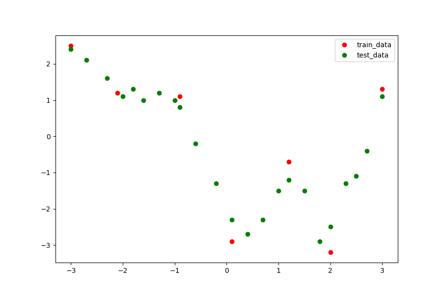
使用原始训练数据做曲线拟合
如图,随着多项式的次数(degree)从2变到6,拟合曲线对训练数据(红色点)的逼近程度越来越高,但是对测试数据的逼近程度却不是如此,特别是degree从4变到6以后,拟合曲线与测试数据的逼近程度反而增大,这就是过拟合现象。
当degree等于8时曲线反而不能完全穿过训练数据,关于此我们前面已有解释。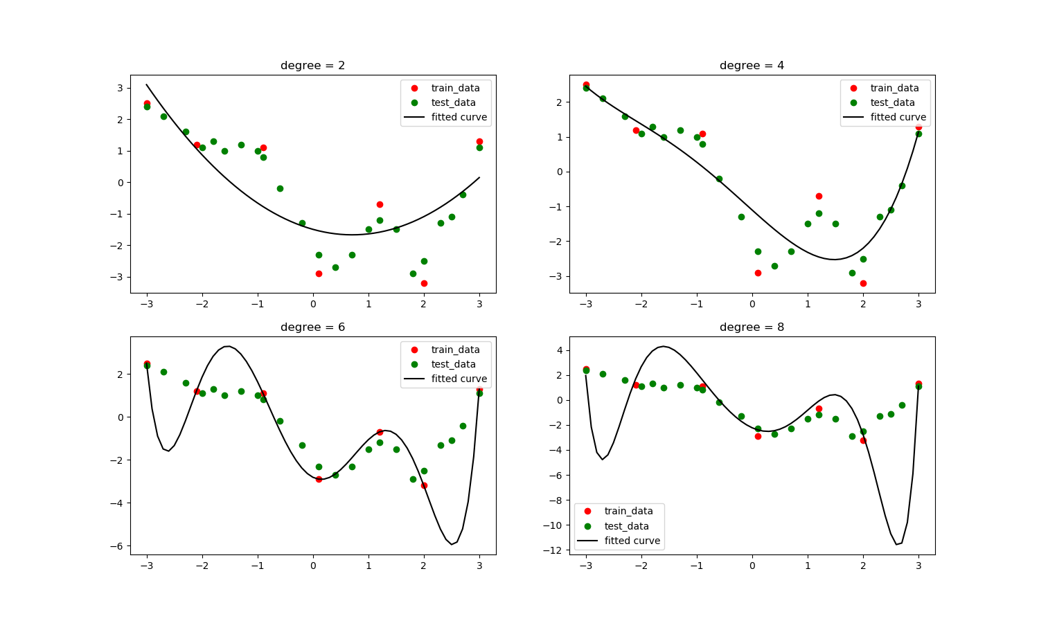
过拟合现象的loss表现
随着模型变大,测试集loss反而开始升高,这就是典型的过拟合现象在loss上的表现。
数据增强
数据增强方式是以训练集中的各个点为基准加上高斯分布的随机数,在其周围构造出一些随机点,这些随机点就是增强后的数据。此例中针对每个训练集中的点构造了20个增强的数据点。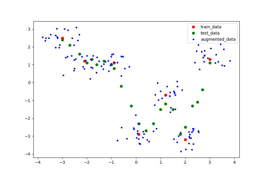
使用增强后的数据做曲线拟合
从图中可以看到,随着模型增大,拟合曲线不仅对训练集的逼近程度越来越高,对测试集的逼近程度也越来越高。这就是数据增强的威力:防止过拟合,提升在测试集上的效果;另外关键是,我们并没有额外地付出数据采集成本。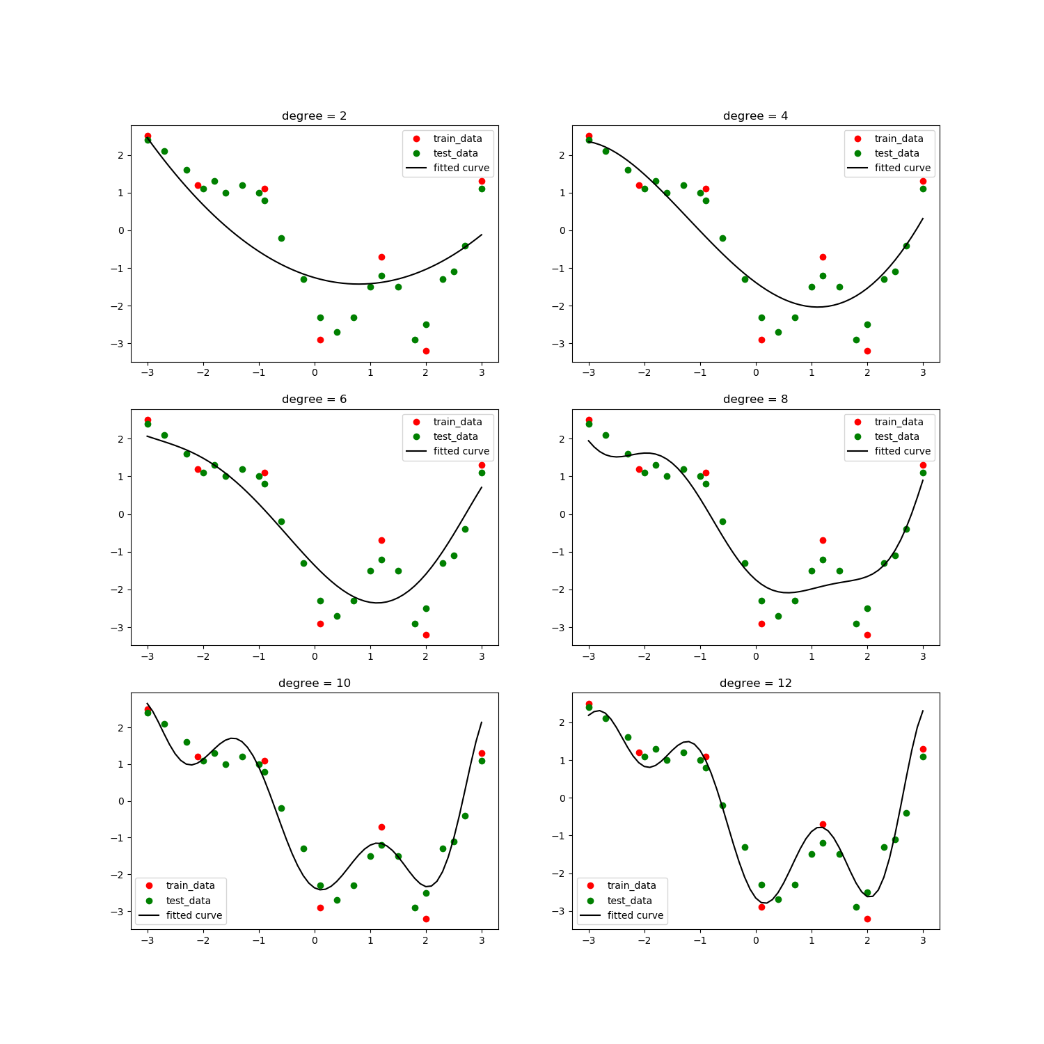
数据增强后的loss表现
从loss上也能看出数据增强带来明显的效果改善,随着模型增大,不仅训练集loss在降低,测试集loss也在不断降低。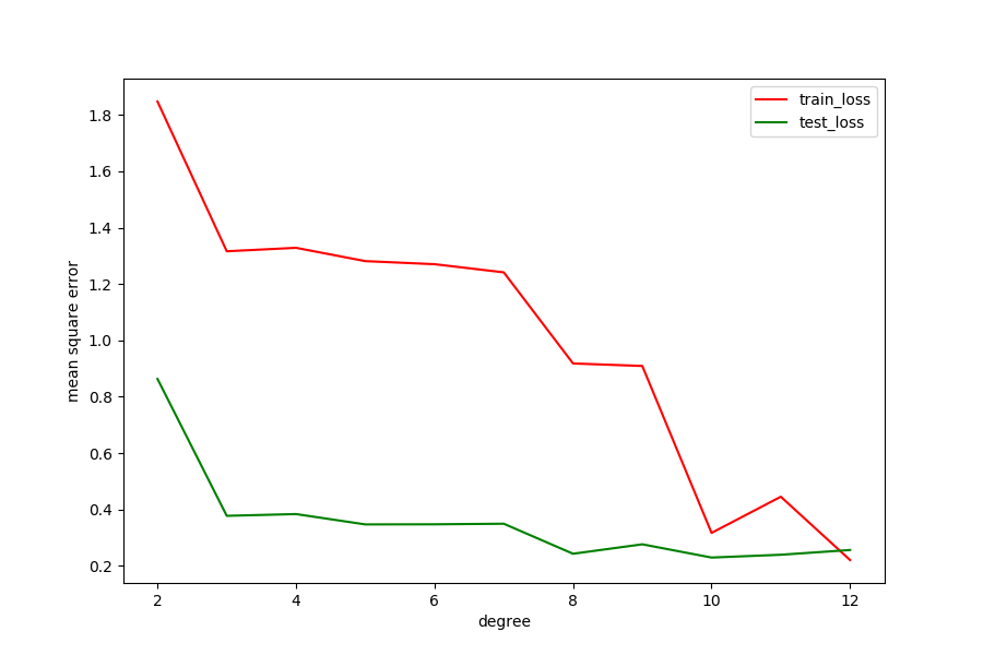


还没有评论,来说两句吧...