Tensorflow2 基本操作字典

Dear 丶 2022-12-18 03:54 201阅读 0赞

**使用方法说明**

明确自己需要查的内容，比如说某个函数 `tf.split` 等，然后直接使用浏览器的查找功能进行查找。

### Tensorflow2 基本操作字典 ###

*  1. 安装与相关资料
 *   *  1.1 安装
     *  1.2 第一个程序
     *  1.3 第二个程序
     *  1.4 相关文档资料
 *  2. tensor 基础
 *   *  2.1 数据类型
     *  2.2 查看变量是不是 tensor
     *  2.3 转换为 tensor
     *  2.4 转换为 tensor 并改变数据类型
     *  2.5 数据类型转换
     *  2.6 tf.Variable（可优化参数）
     *  2.7 查看变量维度
     *  2.8 查看变量是否可以优化 trainable
     *  2.9 创建 tensor 的方法
     *   *  2.9.1 constant 函数
         *  2.9.2 从 numpy 或 list 数据转换
         *  2.9.3 tf.zeros、tf.ones 函数
         *  2.9.4 tf.fill 函数、tf.range函数
         *  2.9.5 tf.random
 *  3. tensor 三大核心操作
 *   *  3.1 索引与切片
     *   *  3.1.1 最基础的索引方法 data\[1\]\[2\]...
         *  3.1.2 简略中括号 data\[1,2,3\]
         *  3.1.3 冒号的使用 data\[start:end\]
         *  3.1.4 冒号的使用 data\[start: end: step\]
         *  3.1.5 负号的使用 data\[-1:\]
         *  3.1.6 省略号的使用 data\[0,...,2\]
     *  3.2 维度变换
     *   *  3.2.1 降维操作 reshape
         *  3.2.2 升维操作 reshape
         *  3.2.3 升维操作 expand\_dims
         *  3.2.4 降维操作 squeeze
         *  3.2.5 -1 的使用
         *  3.2.6 维度调换
     *  3.3 broadcast
     *   *  3.3.1 隐式使用 broadcast 机制
         *  3.3.2 numpy 的 broadcast 机制
         *  3.3.3 显式扩展
         *  3.3.4 Broadcast vs Tile
         *  3.3.5 broadcast 的条件
 *  4. tf 的数学运算
 *  5. tensor 的高阶操作
 *   *  5.1 合并与分割
     *   *  5.1.1 合并 tf.concat
         *  5.1.2 均匀分割 tf.split
         *  5.1.3 堆叠 tf.stack
         *  5.1.4 单个分割 tf.unstack
     *  5.2 数据统计
     *   *  5.2.1 最小值、最大值、平均值、求和
         *  5.2.2 求最值对应的位置
         *  5.2.3 判断相等 tf.equal
         *  5.2.4 去除重复（统计不同种类）
     *  5.3 tensor 排序
     *   *  5.3.1 tf.sort
         *  5.3.2 tf.argsort
         *  5.3.3 tf.math.top\_k
     *  5.4 填充与复制
     *   *  5.4.1 填充相同数字 tf.fill
         *  5.4.2 tf.pad
         *  5.4.3 tf.tile
     *  5.5 张量限幅
     *   *  5.5.1 tf.maximum 与 tf.minimum
         *  5.5.2 根据具体数值进行裁剪 clip\_by\_value
         *  5.5.3 裁剪成最大L2范数 clip\_by\_norm
         *  5.5.4 根据总体范数裁剪 clip\_by\_global\_norm
     *  5.6 高阶操作
     *   *  5.6.1 根据坐标有目的性的选择 tf.where
         *  5.6.2 根据坐标有目的性的更新 tf.scatter\_nd
         *  5.6.3 生成坐标 tf.meshgrid
 *  6. 数据加载
 *   *  6.1 tf.keras.datasets
     *   *  6.1.1 数据集总体介绍
         *  6.1.2 加载方法
     *  6.2 pandas 加载数据集
     *   *  6.2.1 远程加载
         *  6.2.2 本地加载
         *  6.2.3 格式转换
     *  6.3 加载 numpy 数据集
     *  6.4 加载图片
     *   *  6.4.1 下载图片
         *  6.4.2 查看图片
         *  6.4.3 使用 tf.keras.preprocessing 加载数据
     *  6.5 加载文本
 *  7. 总结

# 1. 安装与相关资料 #

## 1.1 安装 ##

环境说明：

*  python3
 *  pip

安装命令（以 2.3.0 版本为例）：

pip install tensorflow -i https://pypi.tuna.tsinghua.edu.cn/simple

查看版本：

pip show tensorflow

如果发现某个镜像速度太慢，考虑其他下载镜像地址:

*  https://mirrors.aliyun.com/pypi/simple/
 *  https://pypi.douban.com/simple/

## 1.2 第一个程序 ##

应用 tensorflow2 中的数学计算。

import tensorflow as tf
    
    A = tf.constant([[1, 2], [3, 4]])
    B = tf.constant([[5, 6], [7, 8]])
    C = tf.matmul(A, B)
    
    print(C)

输出内容：

tf.Tensor(
    [[19 22]
     [43 50]], shape=(2, 2), dtype=int32)

## 1.3 第二个程序 ##

手写数字识别简单例子。

import tensorflow as tf
    
    # 加载数据
    mnist = tf.keras.datasets.mnist
    
    (x_train, y_train), (x_test, y_test) = mnist.load_data()
    x_train, x_test = x_train / 255.0, x_test / 255.0
    model = tf.keras.models.Sequential([
      tf.keras.layers.Flatten(input_shape=(28, 28)),
      tf.keras.layers.Dense(128, activation='relu'),
      tf.keras.layers.Dropout(0.2),
      tf.keras.layers.Dense(10, activation='softmax')
    ])
    
    model.compile(optimizer='adam',
                  loss='sparse_categorical_crossentropy',
                  metrics=['accuracy'])
    
    model.fit(x_train, y_train, epochs=10)
    
    print(model.evaluate(x_test,  y_test, verbose=2))

输出内容包括：

Epoch 1/10
    1875/1875 [==============================] - 3s 2ms/step - loss: 0.2942 - accuracy: 0.9140
    Epoch 2/10
    1875/1875 [==============================] - 3s 2ms/step - loss: 0.1431 - accuracy: 0.9573
    Epoch 3/10
    1875/1875 [==============================] - 3s 1ms/step - loss: 0.1080 - accuracy: 0.9676
    Epoch 4/10
    1875/1875 [==============================] - 3s 1ms/step - loss: 0.0900 - accuracy: 0.9721
    Epoch 5/10
    1875/1875 [==============================] - 3s 1ms/step - loss: 0.0775 - accuracy: 0.9760
    Epoch 6/10
    1875/1875 [==============================] - 3s 2ms/step - loss: 0.0654 - accuracy: 0.9789
    Epoch 7/10
    1875/1875 [==============================] - 3s 2ms/step - loss: 0.0579 - accuracy: 0.9814
    Epoch 8/10
    1875/1875 [==============================] - 3s 2ms/step - loss: 0.0535 - accuracy: 0.9827
    Epoch 9/10
    1875/1875 [==============================] - 3s 2ms/step - loss: 0.0486 - accuracy: 0.9842
    Epoch 10/10
    1875/1875 [==============================] - 3s 2ms/step - loss: 0.0451 - accuracy: 0.9850
    313/313 - 0s - loss: 0.0702 - accuracy: 0.9796
    [0.07019094377756119, 0.9796000123023987]

## 1.4 相关文档资料 ##

*  官网 [API 文档][API] 是最简单直接高效的查询地址
 *  [视频教程][Link 1] 自行选择 B 站的一些视频进行学习
 *  [龙书][Link 2] 由龙龙老师编写的书籍，提供PPT与源码，很值得学习。记得给龙龙老师的github点星星。
 *  龙老师提供的 [付费视频教程][Link 3]  
    \*《深度学习：基于Keras的Pythons
 *

# 2. tensor 基础 #

## 2.1 数据类型 ##

数据类型包括

*  数值类型（int, float, double）
 *  字符类型 （string）
 *  布尔类型（bool）

其中的数值类型常常根据维度数分类：

*  标量(Scalar)。单个的实数，如 1.2, 3.4 等，维度(Dimension)数为 0，shape 为\[ \]。
 *  向量(Vector)。 n n n 个实数的有序集合，通过中括号包裹，如\[1.2\]，\[1.2,3.4\]等，维度数  
    为 1，长度不定，shape 为 \[n\]
 *  矩阵(Matrix)。 n n n 行  m m m 列实数的有限集合。比如 \[ \[1, 2 \], \[3,4\] \]
 *  张量(tensor)。一般把标量、向量和矩阵统称为张量。(都是tensor的对象)

## 2.2 查看变量是不是 tensor ##

import tensorflow as tf
    a = 2
    print(tf.is_tensor(a)) # False
    b = tf.constant(2)
    print(tf.is_tensor(b)) # True

注意 `tf.is_tensor()` 和 `isinstance` 的区别：

import tensorflow as tf
    
    b = tf.constant(2)
    print(tf.is_tensor(b)) # True
    print(isinstance(b, tf.Tensor)) # True
    
    b = tf.Variable(b)
    print(tf.is_tensor(b)) # True
    print(isinstance(b, tf.Tensor)) # False

尽管在 b 已经转化为 `tf.Variable` 类型，但是它本身依然是 tensor类型，但 `isinstance` 函数返回 `False`，所以推荐使用 `tf.is_tensor` 函数。

## 2.3 转换为 tensor ##

import tensorflow as tf
    a = 2
    print(tf.is_tensor(a)) # False
    a = tf.convert_to_tensor(a)
    print(tf.is_tensor(a)) # True

## 2.4 转换为 tensor 并改变数据类型 ##

import tensorflow as tf
    
    a = 123
    a = tf.convert_to_tensor(a, dtype=tf.float32)
    print(a.dtype) # <dtype: 'float32'>

## 2.5 数据类型转换 ##

import tensorflow as tf
    
    a = 123
    
    a = tf.cast(a, dtype=tf.float32)
    print(a.dtype)             # <dtype: 'float32'>
    print(tf.is_tensor(a))     # True
    
    b = [0,1]
    b = tf.cast(b, dtype=tf.bool) 
    print(b.dtype)             # <dtype: 'bool'>
    print(tf.is_tensor(b))     # True

## 2.6 tf.Variable（可优化参数） ##

使用 tf.Variable 修饰某个变量，代表这个变量是可以优化的参数，在循环迭代中会改变这个参数的值达到整体更好的效果。

import tensorflow as tf
    param = 2.4
    param = tf.Variable(param)
    print(tf.is_tensor(param))    # True
    print(param.dtype)            # <dtype: 'float32'>

## 2.7 查看变量维度 ##

import tensorflow as tf
    a = tf.constant(1)
    print(a.ndim)               # 0
    print(a.shape)              # ()
    
    b = tf.constant([1,2,3,4])
    print(b.ndim)               # 1
    print(b.shape)              # (4,)
    
    c = tf.constant([[1,2],[3,4]])
    print(c.ndim)               # 2
    print(c.shape)              # (2,2)

## 2.8 查看变量是否可以优化 trainable ##

import tensorflow as tf
    
    a = tf.constant([1,2,3,4])
    # print(a.trainable) # 运行这行报错 has no attribute 'trainable'
    
    a = tf.Variable(a)
    print(a.trainable)        # True

## 2.9 创建 tensor 的方法 ##

### 2.9.1 constant 函数 ###

import tensorflow as tf
    tf.constant([1,2])

### 2.9.2 从 numpy 或 list 数据转换 ###

import numpy as np
    import tensorflow as tf
    
    ary = np.array([1,2,3])  
    a = tf.convert_to_tensor(ary)
    print(a.dtype)                # <dtype: 'int64'>
    print(tf.is_tensor(a))        # True

### 2.9.3 tf.zeros、tf.ones 函数 ###

import tensorflow as tf
    
    a = tf.zeros([2,3])
    print(a.dtype)               # <dtype: 'float32'> 
    print(tf.is_tensor(a))       # True
    
    b = tf.ones([2,3])
    print(b.dtype)               # <dtype: 'float32'> 
    print(tf.is_tensor(b))       # True

### 2.9.4 tf.fill 函数、tf.range函数 ###

import tensorflow as tf
    
    c = tf.fill([1,2,3],110)
    print(c.dtype)               # <dtype: 'int32'> 
    print(tf.is_tensor(c))       # True
    
    d = tf.range(40)
    print(c.dtype)               # <dtype: 'int32'> 
    print(tf.is_tensor(c))       # True

### 2.9.5 tf.random ###

import tensorflow as tf
    
    # 正泰分布
    a = tf.random.normal([2,3],mean=1,stddev=1)
    print(a.dtype)               # <dtype: 'float32'> 
    print(tf.is_tensor(a))       # True
    
    # 均匀分布
    b = tf.random.uniform([2,3],minval=0,maxval=1)
    print(b.dtype)               # <dtype: 'float32'> 
    print(tf.is_tensor(b))       # True
    
    # 随机打乱
    c = tf.range(50)
    tf.random.shuffle(c)
    print(c.dtype)               # <dtype: 'int32'> 
    print(tf.is_tensor(c))       # True

# 3. tensor 三大核心操作 #

为了解释更加方便，约定

*  \[b, h, w\] 表示 b 张 高为 h，宽为 w 的图片。
 *  \[b, h, w, 3\] 表示 b 张 高为h， 宽为 w 的彩色图片，最后的 \[3\] 表示对应的 RGB 值。
 *  \[50,28,28\] 表示 50 张 28x28 的图片。
 *  \[50,28,28,3\] 表示 50 张 28x28 的彩色图片。

## 3.1 索引与切片 ##

### 3.1.1 最基础的索引方法 data\[1\]\[2\]… ###

import tensorflow as tf
    
    data = tf.random.normal([50,28,28],mean=1,stddev=1)
    # 获得第一张图片最后一个像素点的值
    print(data[0][27][27])
    # 获得第一张图片第一行的所有像素值
    print(data[0][0])
    # 获得第二张图片的像素值矩阵
    print(data[1])

### 3.1.2 简略中括号 data\[1,2,3\] ###

import tensorflow as tf
    
    data = tf.random.normal([50,28,28],mean=1,stddev=1)
    # 获得第一张图片最后一个像素点的值
    print(data[0,27,27])
    # 获得第一张图片第一行的所有像素值
    print(data[0,0])
    # 获得第二张图片的像素值矩阵
    print(data[1])

### 3.1.3 冒号的使用 data\[start:end\] ###

import tensorflow as tf
    
    data = tf.random.normal([50,28,28],mean=1,stddev=1)
    # 查看前五张图片的像素值
    print(data[0:5])
    # 查看第一张图片的第1行到第5行，最后一列的像素值
    print(data[0,:5,27])

### 3.1.4 冒号的使用 data\[start: end: step\] ###

import tensorflow as tf
    
    data = tf.random.normal([50,28,28],mean=1,stddev=1)
    # 查看所有偶数号图片的像素值
    print(data[::2])
    # 查看前一百张图片中所有奇数号的像素值
    print(data[1:100:2])

### 3.1.5 负号的使用 data\[-1:\] ###

import tensorflow as tf
    
    data = tf.random.normal([50,28,28],mean=1,stddev=1)
    # 查看最后一张图片的像素值
    # 等价于 print(data[49])
    print(data[-1])
    # 查看最后一张图片最后一行的像素
    print(data[-1,-1,:])

### 3.1.6 省略号的使用 data\[0,…,2\] ###

import tensorflow as tf
    
    # 最后的 [3] 表示 RGB 像素值
    data = tf.random.normal([50,28,28,3],mean=1,stddev=1)
    #查看第一张图片的 R 值
    print(data[0,:,:,0])
    # 与这个是等价的，省略中间的两个连续的冒号
    print(data[0,...,0])

## 3.2 维度变换 ##

以像素值为例，\[b, h, w, 3\] 表示 b 张高为 h 宽为 w 的 彩色图片，那么进行维度变换的过程中，必须保证像素值 b\*h\*w\*3 的值不变。

### 3.2.1 降维操作 reshape ###

import tensorflow as tf
    
    data = tf.random.normal([50,28,28,3],mean=1,stddev=1)
    # 降维 1
    data1 = tf.reshape(data, [50, 784, 3])
    print(data1.shape)                      # (50, 784, 3)
    
    # 降维 2
    data2 = tf.reshape(data, [50,784*3])
    print(data2.shape)                      # (50, 2352)
    
    # 降维 3
    data3 = tf.reshape(data, [50*784*3])
    print(data3.shape)                     # (117600,)

### 3.2.2 升维操作 reshape ###

升维操作需要注意必须指定维度的先后顺便保证不出错。这次假设图片的尺寸为 128 \* 64

import tensorflow as tf
    
    # 假设 data 是已经经过降维处理，原始图片尺寸是 [128, 64]
    data = tf.random.normal([50,128*64,3],mean=1,stddev=1)
    
    # 升维操作必须保证顺序没弄错
    data1 = tf.reshape(data, [50, 128, 64, 3])
    print(data1.shape)
    
    # 如果顺序弄错结果图片会出问题
    data2 = tf.reshape(data, [50, 64, 128, 3])      # 不能得到降维前的图片
    print(data2.shape)

### 3.2.3 升维操作 expand\_dims ###

expand\_dim 用于增加某个数值为 1 的维度，并指定增加的位置。

import tensorflow as tf
    
    # 原来的图片 [50, h, w, 3] 需要对调成为 [50, 3, h, w]
    data = tf.random.normal([50,128,64,3],mean=1,stddev=1)
    
    # 增加 到 第一个维度
    data1 = tf.expand_dims(data,0)
    print(data1.shape)                    # (1, 50, 128, 64, 3)
    
    # 增加在最后一个位置
    data2 = tf.expand_dims(data,-1)
    print(data2.shape)                    # (50, 128, 64, 3, 1)
    
    # 增加在第二个位置，第三个位置不复说明

### 3.2.4 降维操作 squeeze ###

tf.squeeze 是默认去掉所有值为 1 的维度，与上面的 expand\_dims 对应关系。  
tf.squeeze 也可以去掉指定位置的 1，如果指定位置不是1则会报错。

import tensorflow as tf
    
    # 原来的图片 [50, h, w, 3] 需要对调成为 [50, 3, h, w]
    data = tf.random.normal([1,50,1,128,1,64,3,1],mean=1,stddev=1)
    
    # 默认却去掉所有为 1 的维度
    data1 = tf.squeeze(data)
    print(data1.shape)                         # (50, 128, 64, 3)
    
    # 去掉下标为 0 而数值为 1 的维度
    data2 = tf.squeeze(data,[0])
    print(data2.shape)                        # (50, 1, 128, 1, 64, 3, 1)
    
    # 去掉下标为 2 或 4 且数值为 1 的维度
    data3 = tf.squeeze(data, [2,4])
    print(data3.shape)                        # (1, 50, 128, 64, 3, 1) # (50, 128, 64, 3)

### 3.2.5 -1 的使用 ###

前面已经说明总值不变，所以如果指定其他值，可以允许出现一个且最多一个 `-1` ，自行计算值。

import tensorflow as tf
    
    data = tf.random.normal([50,28,28,3],mean=1,stddev=1)
    # 降维 1
    data1 = tf.reshape(data, [50, -1, 3])
    print(data1.shape)                      # (50, 784, 3)
    
    # 降维 2
    data2 = tf.reshape(data, [50, 784, -1])
    print(data2.shape)        
    
    # 从 data1 升维 1
    data3 = tf.reshape(data1, [50,-1,28,3])
    print(data3.shape)        
    
    # 从 data1 升维 2
    data4 = tf.reshape(data1, [50,28,28,-1])
    print(data4.shape)

### 3.2.6 维度调换 ###

比如说 对于原来的图片 \[50, 128, 64, 3\] 如果需要把行与列进行对调，则需要对维度进行调换操作。用到的是 tf.transpose 函数。

tf.transpose 函数的用法与 reshape 很像，但是第二个参数对应的是现在的维度与原来的维度一 一对应关系。比如说下面的：

*  tf.transpose(data, \[0, 3, 1, 2\]) 表示把以前 第4个维度换到现在的第2个维度，原来的第2个维度换到第3个维度，原来的第3个维度换到第4个维度。
 *  tf.transpose(data1, \[0, 2, 3, 1\]) 表示把以前 第3个维度换到现在的第2个维度，把原来的第4个维度换到现在的第3个维度，把原来的第2个维度换到第4个维度。

import tensorflow as tf
    
    # 原来的图片 [50, h, w, 3] 需要对调成为 [50, 3, h, w]
    data = tf.random.normal([50,128,64,3],mean=1,stddev=1)
    
    data1 = tf.transpose(data, [0,3,1,2])
    print(data1.shape)          # (50, 3, 128, 64)
    
    # 再从 [50, 3, 128, 64]
    data2 = tf.transpose(data1, [0,2,3,1])
    print(data2.shape)          # (50, 128, 64, 3)

## 3.3 broadcast ##

broadcasting 是一个自动扩展机制，能够对一些变量进行扩展以便于完成计算。它最神奇的地方在于，“看起来扩展了，但并未增加内存消耗”。仔细想想应该是使用类似于 C 语言强大的指针可以完成很多事情一样。

因为 broadcasting 的扩展虽然不占额外的内存，但是它扩展的部分本身就存在，扩展的值是一样的值。比如说，在 numpy 中 矩阵的规格为 \[3, 4\] 时，与 矩阵规格 \[1, 4\] 是不能进行加法运算的，但是 tensorflow 中通过broadcasting 即可完成这个操作。

### 3.3.1 隐式使用 broadcast 机制 ###

import tensorflow as tf
    
    a = tf.fill([3,4],5)
    b = tf.fill([1,4],4)
    c = a + b
    print(c)

输出内容为：

tf.Tensor(
    [[9 9 9 9]
     [9 9 9 9]
     [9 9 9 9]], shape=(3, 4), dtype=int32)

### 3.3.2 numpy 的 broadcast 机制 ###

在 numpy 中也有 broadcast 机制，比如：

import numpy as np 
     
    a = np.array([[ 0, 0, 0],
               [10,10,10],
               [20,20,20],
               [30,30,30]])
    b = np.array([1,2,3])
    print(a + b)

输出内容为：

[[ 1  2  3]
     [11 12 13]
     [21 22 23]
     [31 32 33]]

### 3.3.3 显式扩展 ###

import tensorflow as tf
    
    b = tf.constant([[1,2,3,4]])
    b = tf.broadcast_to(b,[3,4])
    print(b)

输出内容：

tf.Tensor(
    [[1 2 3 4]
     [1 2 3 4]
     [1 2 3 4]], shape=(3, 4), dtype=int32)

### 3.3.4 Broadcast vs Tile ###

同样的 numpy 也有 tile 函数，这里不介绍 numpy 的对应内容。

tf.tile 配合 tf.expand\_dims 可以达到 broadcast 的效果，但是 broadcast 的最大优点在于 不占用额外内存空间。

tf.tile + tf.expand\_dims 实现 broadcast 的例子

import tensorflow as tf
    
    a = tf.constant([[1,2,3,4],[5,6,7,8],[9,10,11,12]])
    print('a.shape:',a.shape)
    
    b = tf.constant([1,2,3,4])
    print('b.shape:',b.shape)
    
    b = tf.expand_dims(b, [0])
    print('after expanding, b.shape:',b.shape)
    
    b = tf.tile(b,[3,1])
    print('after tiling , b.shape:',b.shape)
    print(b)
    
    print(a + b)

输出内容：

a.shape: (3, 4)
    b.shape: (4,)
    after expanding, b.shape: (1, 4)
    after tiling, b.shape: (3, 4)
    tf.Tensor(
    [[1 2 3 4]
     [1 2 3 4]
     [1 2 3 4]], shape=(3, 4), dtype=int32)
    tf.Tensor(
    [[ 2  4  6  8]
     [ 6  8 10 12]
     [10 12 14 16]], shape=(3, 4), dtype=int32)

如果直接使用 tf,broadcast 机制就非常简单，如下：

import tensorflow as tf 
    a = tf.constant([[1,2,3,4],[5,6,7,8],[9,10,11,12]])
    b = tf.constant([1,2,3,4])
    print(a+b)

### 3.3.5 broadcast 的条件 ###

矩阵 a 与 矩阵 b 进行运算时，以加法为例，默认使用 broadcast 时需要满足一些条件。

假设 a.shape = ( m 1 , m 2 , . . . , m k m\_1, m\_2, ..., m\_k m1,m2,...,mk)，b.shape = ( n 1 , n 2 , . . . , n j n\_1,n\_2,...,n\_j n1,n2,...,nj)，其中  k > = j k>=j k>=j，从右边到左边必须保证  n j − i n\_\{j-i\} nj−i =  m k − i m\_\{k-i\} mk−i ，如果存在正整数  i i i 使得等式  n j − i n\_\{j-i\} nj−i =  m k − i m\_\{k-i\} mk−i 不成立而且 m k − i 不 等 于 1 m\_\{k-i\}不等于1 mk−i不等于1，则说明不能进行 broadcast 操作。

例子如下：

a.shape + b.shape：

*  \[1,2,3,4\] + \[4\] 可以运算
 *  \[1,2,3,4\] + \[1\] 可以运算
 *  \[1,2,3,4\] + \[3, 4\] 可以运算
 *  \[1,2,3,4\] + \[1, 4\] 可以运算
 *  \[1,2,3,4\] + \[1,3,4\] 可以运算
 *  \[1,2,3,4\] + \[1,1,3,4\] 可以运算
 *  \[1,2,3,4\] + \[2,4\] 不可以运算
 *  \[1,2,3,4\] + \[2\] 不可以运算
 *  \[1,2,3,4\] + \[2,2,3,4\] 可以运算

# 4. tf 的数学运算 #

运算符包括

*  \+ - \* /
 *  \*\* pow
 *  sqrt
 *  // (取整) % （取余）
 *  @ （矩阵乘法，a@b）
 *  exp （以 e 为底的指数函数, tf.exp(x))
 *  log (以 e 为底的对数函数, tf.math.log(x) )

import tensorflow as tf
    
    x = tf.ones([4,2])
    w = tf.ones([2,1])
    b = tf.constant(0.1)
    
    print(x@w+b)

输出内容为：

tf.Tensor(
    [[2.1]
     [2.1]
     [2.1]
     [2.1]], shape=(4, 1), dtype=float32)

# 5. tensor 的高阶操作 #

## 5.1 合并与分割 ##

### 5.1.1 合并 tf.concat ###

concat 的 axis 参数表示以某个维度为标准进行合并，其他维度上的数目必须相同才能合并。合并的过程并不会改变维度。

import tensorflow as tf
    
    # 50 张 28x28 的图片与 30 张 28x28 的图片合并一个 tensor
    
    a = tf.random.normal([50,28,28],mean=1,stddev=1)  
    b = tf.random.normal([30,28,28],mean=1,stddev=1)
    
    result = tf.concat([a, b], axis=0)
    print(result.shape)     # (80, 28, 28)
    
    c = tf.random.normal([60,28,28],mean=1,stddev=1)
    
    result = tf.concat([a, b, c], axis=0)
    print(result.shape)     # (140, 28, 28)

50 张分别只包含 r / g / b 数据的 tensor 合并起来

import tensorflow as tf
    
    # 50 张分别只包含 r / g / b 数据的 tensor 合并起来
    r = tf.random.normal([50,28,28,1],mean=1,stddev=1)
    g = tf.random.normal([50,28,28,1],mean=1,stddev=1)
    b = tf.random.normal([50,28,28,1],mean=1,stddev=1)
    
    result = tf.concat([r, g, b], axis=3)
    print(result.shape)     # (50, 28, 28, 3)

### 5.1.2 均匀分割 tf.split ###

import tensorflow as tf
    
    # 把 rgb 图片分别分割成 r g b 三个 tensor
    rgb = tf.random.normal([50,28,28,3],mean=1,stddev=1)
    
    r,g,b = tf.split(rgb,num_or_size_splits=3, axis=3)
    
    print('r.shape:',r.shape)        # r.shape: (50, 28, 28, 1)
    print('g.shape:',g.shape)        # g.shape: (50, 28, 28, 1)
    print('b.shape:',b.shape)        # b.shape: (50, 28, 28, 1)

### 5.1.3 堆叠 tf.stack ###

如果三个代表不同含义的tensor需要组合的话，需要添加新的维度时使用 stack 比较方便。

import tensorflow as tf
    
    # 50 张 分别代表图片的 r g b 值 的 tensor，合并时指定添加位置
    r = tf.random.normal([50,28,28],mean=1,stddev=1)
    g = tf.random.normal([50,28,28],mean=1,stddev=1)
    b = tf.random.normal([50,28,28],mean=1,stddev=1)
    
    result = tf.stack([r,g,b],axis=3)
    print(result.shape)     # (140, 28, 28, 3)
    
    result2 = tf.stack([r,g,b],axis=1)
    print(result2.shape)     # (140, 3, 28, 28)

### 5.1.4 单个分割 tf.unstack ###

跟 tf.split 有些类似，可以理解为 tf.stack 的逆过程。

import tensorflow as tf
    
    # 把 rgb 图片分别分割成 r g b 三个 tensor
    rgb = tf.random.normal([50,28,28,3],mean=1,stddev=1)
    
    results = tf.unstack(rgb,axis=3) 
    print(len(results))                          # 3
    print(results[0].shape)                      # (50, 28, 28)
    
    results2 = tf.unstack(rgb, axis=0)
    print(len(results2))                          # 50
    print(results2[0].shape)                      # (28, 28, 3)

## 5.2 数据统计 ##

### 5.2.1 最小值、最大值、平均值、求和 ###

默认是全部数据进行求解

import tensorflow as tf
    
    a = tf.constant([1,2,3,4])
    print(tf.reduce_mean(a))             # tf.Tensor(2, shape=(), dtype=int32)
    print(tf.reduce_max(a))              # tf.Tensor(4, shape=(), dtype=int32)
    print(tf.reduce_sum(a))              # tf.Tensor(10, shape=(), dtype=int32)
    b = tf.constant([[1,2],[3,4]])
    print(tf.reduce_mean(b))             # tf.Tensor(2, shape=(), dtype=int32)
    print(tf.reduce_max(b))              # tf.Tensor(4, shape=(), dtype=int32)

如果需要按行统计的话，需要指定 axis = 1  
如果需要按列统计的话，需要指定 axis = 0

import tensorflow as tf
    
    c = tf.random.normal([2,3])      # 2 行 3 列
    print(c)
    
    # mean, max, sum 用法一样
    print(tf.reduce_min(c, axis=0)) # [3 个数]
    print(tf.reduce_min(c, axis=1)) # [2 个数]

输出内容：

tf.Tensor(
    [[-0.77924424 -1.3409568   0.15045725]
     [ 0.6147348   0.34684792 -1.1834606 ]], shape=(2, 3), dtype=float32)
    tf.Tensor([-0.77924424 -1.3409568  -1.1834606 ], shape=(3,), dtype=float32)
    tf.Tensor([-1.3409568 -1.1834606], shape=(2,), dtype=float32)

### 5.2.2 求最值对应的位置 ###

上面的函数返回的是最值，当所需要的是返回最值对应的位置时，需要用到 tf.argmax / argmin 函数。

import tensorflow as tf
    
    c = tf.random.normal([2,3])
    print(c)
    
    print(tf.argmin(c))
    print(tf.argmax(c))
    
    print(tf.argmin(c, axis=1))

输出内容为：

tf.Tensor(
    [[ 1.0865854   1.49058     1.4004668 ]
    [-0.4294602  -1.1244454   0.49177092]], shape=(2, 3), dtype=float32)
    tf.Tensor([1 1 1], shape=(3,), dtype=int64)
    tf.Tensor([0 0 0], shape=(3,), dtype=int64)
    tf.Tensor([0 1], shape=(2,), dtype=int64)

### 5.2.3 判断相等 tf.equal ###

同样地，tensor 也可以比较大小是否相等。

import tensorflow as tf
    
    a = tf.range(6)
    b = tf.range(6)
    
    print(tf.equal(a, b))             # tf.Tensor([ True True True True True True], shape=(6,), dtype=bool)

当然，如果是矩阵的话返回的也是矩阵格式。

### 5.2.4 去除重复（统计不同种类） ###

使用 tf.unique 函数返回的是一个长度为2的列表，第一个是去重后的列表，第二个是去重前的每个数与去重后的每个数之间的对应位置关系。(即索引号)

import tensorflow as tf
    a = tf.constant([1,2,1,3,1,4])
    b1,b2 = tf.unique(a)
    
    # b1 表示去重后的数组
    # b2 表示去重前的数与去重后的数的索引 (对应位置关系)
    # 比如说去重前 a[0] 对应去重后的 b1[0] 去重前的 a[2] 对应去重后的 b1[0] 等等
    print('b1:',b1)            # b1: tf.Tensor([1 2 3 4], shape=(4,), dtype=int32)
    print('b2:',b2)            # b2: tf.Tensor([0 1 0 2 0 3], shape=(6,), dtype=int32)

根据完成去重后得到的两个列表b1,b2，也可以通过随机索引得到去重前的列表。

import tensorflow as tf
    
    b1 = tf.constant([1,2,3,4])
    b2 = tf.constant([0,1,0,2,0,3])
    
    a = tf.gather(b1, b2)
    print(a)            # tf.Tensor([1 2 1 3 1 4], shape=(6,), dtype=int32)

## 5.3 tensor 排序 ##

### 5.3.1 tf.sort ###

默认情况下是从小到大排序，需要指定 direction 参数来实现从大到小排序。具体操作如下：

import tensorflow as tf
    
    a = tf.range(10)
    
    # 随机打乱
    a = tf.random.shuffle(a) 
    
    # 默认排序是 从小到大
    b = tf.sort(a)
    print(b)                                # [0, 1, 2, 3, 4, 5, 6, 7, 8,9]
    
    # 指定从大到小排序
    c = tf.sort(a, direction='DESCENDING')
    print(c)                                # [9, 8, 7, 6, 5, 4, 3, 2, 1, 0]

当维度 > 1 时，可以指定排序的方式，即指定 index 参数，以二维为例，可以有两种排序方法：

import tensorflow as tf
    
    a = tf.constant([
        [1, 2, 3],
        [7, 9, 8],
        [10, 12, 11],
        [6, 5, 4],
    ])
    # 默认情况下 axis = -1，即最后一个维度
    print(tf.sort(a))
    print(tf.sort(a,axis=0))
    print(tf.sort(a,axis=1))

输出内容如下，注意对应关系。

tf.Tensor(
    [[ 1  2  3]
     [ 7  8  9]
     [10 11 12]
     [ 4  5  6]], shape=(4, 3), dtype=int32)
    tf.Tensor(
    [[ 1  2  3]
     [ 6  5  4]
     [ 7  9  8]
     [10 12 11]], shape=(4, 3), dtype=int32)
    tf.Tensor(
    [[ 1  2  3]
     [ 7  8  9]
     [10 11 12]
     [ 4  5  6]], shape=(4, 3), dtype=int32)

### 5.3.2 tf.argsort ###

和 tf.sort 用法差不多，但它返回的是 排序后 与排序前的对应关系。

import tensorflow as tf
    
    a = tf.constant([
        [1, 2, 3],
        [7, 9, 8],
        [10, 12, 11],
        [6, 5, 4],
    ])
    # 默认情况下 axis = -1，即最后一个维度
    print(tf.sort(a))
    print(tf.argsort(a))

输出内容为：

tf.Tensor(
    [[ 1  2  3]
     [ 7  8  9]
     [10 11 12]
     [ 4  5  6]], shape=(4, 3), dtype=int32)
    tf.Tensor(
    [[0 1 2]
     [0 2 1]
     [0 2 1]
     [2 1 0]], shape=(4, 3), dtype=int32)

### 5.3.3 tf.math.top\_k ###

tf.math.top\_k 函数默认参数 k = 1，返回两个数列，第一个数列返回 top 值，第二个数列返回 top 值对应的索引。

import tensorflow as tf
    
    a = tf.constant([
        [1, 2, 3],
        [7, 9, 8],
        [10, 12, 11],
        [6, 5, 4],
    ])
    
    top_k, indies = tf.math.top_k(a)
    print(top_k)
    print(indies)

输出为：

tf.Tensor(
    [[ 3]
     [ 9]
     [12]
     [ 6]], shape=(4, 1), dtype=int32)
    tf.Tensor(
    [[2]
     [1]
     [1]
     [0]], shape=(4, 1), dtype=int32)

指定 k 参数值

import tensorflow as tf
    
    a = tf.constant([
        [1, 2, 3],
        [7, 9, 8],
        [10, 12, 11],
        [6, 5, 4],
    ])
    
    top_k, indies = tf.math.top_k(a,k=2)
    print(top_k)
    print(indies)

输出内容为：

tf.Tensor(
    [[ 3  2]
     [ 9  8]
     [12 11]
     [ 6  5]], shape=(4, 2), dtype=int32)
    tf.Tensor(
    [[2 1]
     [1 2]
     [1 2]
     [0 1]], shape=(4, 2), dtype=int32)

## 5.4 填充与复制 ##

### 5.4.1 填充相同数字 tf.fill ###

前面 创建tensor 的时候提到过 tf.fill 方法，使用方法简单，但只是在创建 tensor 的时候使用，不能对 tensor 进行修改等操作。

import tensorflow as tf
    
    tf.fill([2,4,3],9)

输出内容为：

tf.Tensor(
    [[[9 9 9]
      [9 9 9]
      [9 9 9]
      [9 9 9]]
    
     [[9 9 9]
      [9 9 9]
      [9 9 9]
      [9 9 9]]], shape=(2, 4, 3), dtype=int32)

### 5.4.2 tf.pad ###

和前端css 属性中的 `padding` 有点关联，css 的时候指定左边间距 `padding-left: 2px` 等等与 tf.pad 参数很相似，具体如例：

t = tf.constant([[1, 2, 3], [4, 5, 6]])
    paddings = tf.constant([[1, 1,], [2, 2]])
    # 'constant_values' is 0.
    # rank of 't' is 2.
    print(tf.pad(t, paddings, "CONSTANT"))  # [[0, 0, 0, 0, 0, 0, 0],
                                            # [0, 0, 1, 2, 3, 0, 0],
                                            # [0, 0, 4, 5, 6, 0, 0],
                                            # [0, 0, 0, 0, 0, 0, 0]]
    # 使用 reflect 反射（注意其中的对应关系）（点对称关系）
    print(tf.pad(t, paddings, "REFLECT"))  # [[6, 5, 4, 5, 6, 5, 4],
                                           # [3, 2, 1, 2, 3, 2, 1],
                                           # [6, 5, 4, 5, 6, 5, 4],
                                           # [3, 2, 1, 2, 3, 2, 1]]
    
    # 对称（线对称关系）
    print(tf.pad(t, paddings, "SYMMETRIC"))  # [[2, 1, 1, 2, 3, 3, 2],
                                             # [2, 1, 1, 2, 3, 3, 2],
                                             # [5, 4, 4, 5, 6, 6, 5],
                                             # [5, 4, 4, 5, 6, 6, 5]]

### 5.4.3 tf.tile ###

对于 tf.tile(input, multiples) ，multiples 决定对输入数据的各位维度的复制次数。对于输入数据shape为 \[ a 1 , a 2 , a 3 , . . . , a i a\_1,a\_2,a\_3,...,a\_i a1,a2,a3,...,ai\] ，当 multiples = \[ m 1 , m 2 , m 3 , . . . , m i m\_1,m\_2,m\_3,...,m\_i m1,m2,m3,...,mi\] 时，使用 tile 函数得到的数据的 shape 为 \[ a 1 ∗ m 1 , a 2 ∗ m 2 , . . . , a i ∗ m i a\_1\*m\_1,a\_2\*m\_2,...,a\_i\*m\_i a1∗m1,a2∗m2,...,ai∗mi\] 。

填充方法也非常简单，就是将对应维度的数据复制对应的倍数即可。

import tensorflow as tf
    
    # [2, 3]
    a = tf.constant([[1,2,3],
                     [4,5,6]])
                     
    # 输出规格为 [2, 6]
    print(tf.tile(a, [1,2]))
    
    # 输出规格为 [4, 3]
    print(tf.tile(a, [2,1]))

输出内容为：

tf.Tensor(
    [[1 2 3 1 2 3]
     [4 5 6 4 5 6]], shape=(2, 6), dtype=int32)
    tf.Tensor(
    [[1 2 3]
     [4 5 6]
     [1 2 3]
     [4 5 6]], shape=(4, 3), dtype=int32)

## 5.5 张量限幅 ##

### 5.5.1 tf.maximum 与 tf.minimum ###

首先介绍这两个函数的用法再说明更复杂的内容。

*  tf.maximum(x, y) 如果是两个数值进行比较，返回其中较大的数；如果是一个数列 `list` 与一个数值`num` 进行比较，则将数列中 `小于` 这个数值 `num` 的数替换成 `num` 并返回，保证数列中最小值为 `num`。
 *  tf.minimum(x,y) 如果两个数值进行比较，返回较小的数；如果是一个数列 `list` 与 一个数值 `num` 进行比较，则将数列中 `大于` 这个数值 `num` 的数替换成 `num` 并返回，保证数列中最大值为 `num`。

import tensorflow as tf
    
    print(tf.maximum(5,6))                    # 6
    
    print(tf.minimum(5,6))                    # 5
    
    a = tf.range(10)
    print(tf.maximum(a,5))                    # [5 5 5 5 5 5 6 7 8 9]
    print(tf.minimum(a,5))                    # [0 1 2 3 4 5 5 5 5 5]
    
    print(tf.maximum(5, a))                    # [5 5 5 5 5 5 6 7 8 9]
    print(tf.minimum(5, a))                    # [0 1 2 3 4 5 5 5 5 5]

这两个函数从某种意义上来讲也是一种裁剪，tf.maximum 裁剪大于某个数值的部分，并把小于这个数值的都替换掉；而tf.minimum 则是裁剪小于某个数的部分，并把大于这个数值的都替换掉。

### 5.5.2 根据具体数值进行裁剪 clip\_by\_value ###

tf.maximum 与 tf.minimum 是取数列的两边，而 tf.clip\_by\_value 则是取数列的中间。  
函数参数包括原数据，maximum 和 minimum ，裁剪中间的部分。

import tensorflow as tf
    
    a = tf.range(10)
    
    print(tf.clip_by_value(a, 2,8))           # [2 2 2 3 4 5 6 7 8 8]

### 5.5.3 裁剪成最大L2范数 clip\_by\_norm ###

clip\_by\_norm 将输入张量值剪辑为最大L2范数。

`clip_norm` 参数可以认为是裁剪缩放尺度，需要根据实际情况而定。

import tensorflow as tf
    
    some_nums = tf.constant([[1, 2, 3, 4, 5]], dtype=tf.float32)
    print(tf.clip_by_norm(some_nums, 1.0))           # [[0.13483998 0.26967996 0.40451992 0.5393599 0.6741999 ]]
    print(tf.clip_by_norm(some_nums, 2.0))           # [[0.26967996 0.5393599 0.80903983 1.0787199 1.3483998 ]]

### 5.5.4 根据总体范数裁剪 clip\_by\_global\_norm ###

clip\_by\_global\_norm 用范数之和的比值剪除多个张量的值。

返回两个变量：global\_norm 和 list\_clipped。其中global\_norm 是进行总体裁剪过的新 norm ，而list\_clipper 是原来的总体范数 global\_norm。

在梯度下降的过程中，即保持总体的方向不变，整体的缩放的比例相同。

这里使用的是 龙老师的例子，具体地址为 [https://github.com/dragen1860/Deep-Learning-with-TensorFlow-book][https_github.com_dragen1860_Deep-Learning-with-TensorFlow-book]

可以直接复制粘贴运行一下查看效果，然后再查看源码，定位到 \`tf.clip\_by\_global\_norm(grads, 15) 处，把附近的一些注解去掉，再次运行查看效果。

也可以考虑把 `tf.clip_by_global_norm(grads, 15)` 参数 `15` 换成其他数字试试。

import  tensorflow as tf
    from    tensorflow import keras
    from    tensorflow.keras import datasets, layers, optimizers
    import  os
    
    os.environ['TF_CPP_MIN_LOG_LEVEL']='2'
    print(tf.__version__)
    
    (x, y), _ = datasets.mnist.load_data()
    x = tf.convert_to_tensor(x, dtype=tf.float32) / 50.
    y = tf.convert_to_tensor(y)
    y = tf.one_hot(y, depth=10)
    print('x:', x.shape, 'y:', y.shape)
    train_db = tf.data.Dataset.from_tensor_slices((x,y)).batch(128).repeat(30)
    x,y = next(iter(train_db))
    print('sample:', x.shape, y.shape)
    # print(x[0], y[0])
    
    
    
    def main():
    
        # 784 => 512
        w1, b1 = tf.Variable(tf.random.truncated_normal([784, 512], stddev=0.1)), tf.Variable(tf.zeros([512]))
        # 512 => 256
        w2, b2 = tf.Variable(tf.random.truncated_normal([512, 256], stddev=0.1)), tf.Variable(tf.zeros([256]))
        # 256 => 10
        w3, b3 = tf.Variable(tf.random.truncated_normal([256, 10], stddev=0.1)), tf.Variable(tf.zeros([10]))
    
    
    
        optimizer = optimizers.SGD(lr=0.01)
    
    
        for step, (x,y) in enumerate(train_db):
    
            # [b, 28, 28] => [b, 784]
            x = tf.reshape(x, (-1, 784))
    
            with tf.GradientTape() as tape:
    
                # layer1.
                h1 = x @ w1 + b1
                h1 = tf.nn.relu(h1)
                # layer2
                h2 = h1 @ w2 + b2
                h2 = tf.nn.relu(h2)
                # output
                out = h2 @ w3 + b3
                # out = tf.nn.relu(out)
    
                # compute loss
                # [b, 10] - [b, 10]
                loss = tf.square(y-out)
                # [b, 10] => [b]
                loss = tf.reduce_mean(loss, axis=1)
                # [b] => scalar
                loss = tf.reduce_mean(loss)
    
    
    
            # compute gradient
            grads = tape.gradient(loss, [w1, b1, w2, b2, w3, b3])
            # print('==before==')
            # for g in grads:
            # print(tf.norm(g))
            
            grads,  _ = tf.clip_by_global_norm(grads, 15)
    
            # print('==after==')
            # for g in grads:
            # print(tf.norm(g))
            # update w' = w - lr*grad
            optimizer.apply_gradients(zip(grads, [w1, b1, w2, b2, w3, b3]))
    
    
    
            if step % 100 == 0:
                print(step, 'loss:', float(loss))
    
    if __name__ == '__main__':
        main()

## 5.6 高阶操作 ##

### 5.6.1 根据坐标有目的性的选择 tf.where ###

tf.where 函数返回的是满足特定条件的数据对应的坐标。

单个参数的时候，需要保证这个参数为 bool 类型的。

例1

import tensorflow as tf
    tf.where([True, False, False, True])

很明显索引为0和索引为3对应的数为 True。

输出内容为

<tf.Tensor: shape=(2, 1), dtype=int64, numpy=
    array([[0],
           [3]])>

例2

import tensorflow as tf
    a = tf.constant([
                        [
                            [True, False], 
                            [False, True], 
                            [True, True]
                        ]
                    ])
    print(a.shape)  # [1, 3, 2]
    tf.where(a)

输入数据shape 为\[1,3,2\]，总共有四个 True，所以应该返回四个坐标。

输出内容为

(1, 3, 2)
    <tf.Tensor: shape=(4, 3), dtype=int64, numpy=
    array([[0, 0, 0],
           [0, 1, 1],
           [0, 2, 0],
           [0, 2, 1]])>

例3

import tensorflow as tf
    
    a = tf.constant(
                    [[-2.2987595, -0.80869454,  0.44529352],
                     [-0.29707265, -0.4740697,  1.1752412 ],
                     [-0.65937036,  0.00989216,  0.11833031]])
    
    print(a)
    
    mask = a>0
    print(mask)
    
    # 取得 大于 0 的数值
    nums = tf.boolean_mask(a, mask)
    print(nums)
    
    # 找到对应的坐标 
    indices = tf.where(mask)
    print(indices)
    
    # 结合 gather_nd 根据坐标从原数据中进行采样
    # 其实就是原来数据中大于0的数
    data = tf.gather_nd(a, indices)
    print(data)

三个参数时，tf.where(mask, x, y)

例4

如果 x 和 y 具有相同 shape，然后根据 mask\[i\] 来绝对返回 x\[i\] 还是 y\[i\]。

import tensorflow as tf
    tf.where([True, False, False, True], [1,2,3,4], [100,200,300,400])

mask\[0\] 为 True，所以选择 x\[0\] 即 1，mask\[1\] 为 False ，所以选择y\[1\] …  
输出内容如下：

<tf.Tensor: shape=(4,), dtype=int32, numpy=array([  1, 200, 300,   4], dtype=int32)>

例5

import tensorflow as tf
    tf.where([True, False, False, True], 1,400)

输出内容为：

<tf.Tensor: shape=(4,), dtype=int32, numpy=array([  1, 400, 400,   1], dtype=int32)>

例6

当 x 和 y 的 shape 不同时，比如：

import tensorflow as tf
    tf.where([True, False, False, True], [1,2,3,4], [100])

输出内容为：

<tf.Tensor: shape=(4,), dtype=int32, numpy=array([  1, 100, 100,   4], dtype=int32)>

### 5.6.2 根据坐标有目的性的更新 tf.scatter\_nd ###

tf.scatter\_nd(indices, updates, shape) 根据坐标有目的更新。

例1

如下图所示，首先指定的shape 决定了生成数据的 shape，这个例子中 shape = 8，所以输出数据的shape 为 8，updates 总共有四个，所以 indices 需要指定把这三个数安插在哪个位置，例子四个数对应的索引是 4,3，1, 7 所以安插完成后 update 数字对应的位置即 4 3 1 7.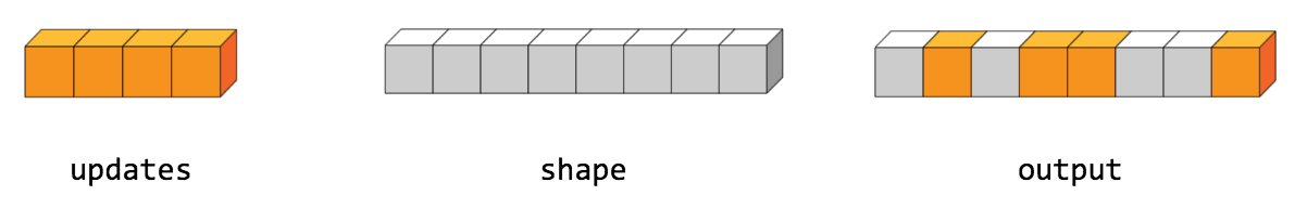  
![在这里插入图片描述][watermark_type_ZmFuZ3poZW5naGVpdGk_shadow_10_text_aHR0cHM6Ly9ibG9nLmNzZG4ubmV0L3NtaWxleWFuOQ_size_16_color_FFFFFF_t_70_pic_center]

import tensorflow as tf
    
    indices = tf.constant([[4], [3], [1], [7]])
    updates = tf.constant([9, 10, 11, 12])
    shape = tf.constant([8])
    scatter = tf.scatter_nd(indices, updates, shape)
    print(scatter)

例 2

理解方法和上面相同。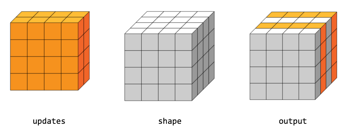  
![在这里插入图片描述][watermark_type_ZmFuZ3poZW5naGVpdGk_shadow_10_text_aHR0cHM6Ly9ibG9nLmNzZG4ubmV0L3NtaWxleWFuOQ_size_16_color_FFFFFF_t_70_pic_center 1]

import tensorflow as tf
    
    indices = tf.constant([[0], [2]])
    updates = tf.constant([[[5, 5, 5, 5], [6, 6, 6, 6],
                            [7, 7, 7, 7], [8, 8, 8, 8]],
                           [[5, 5, 5, 5], [6, 6, 6, 6],
                            [7, 7, 7, 7], [8, 8, 8, 8]]])
    shape = tf.constant([4, 4, 4])
    scatter = tf.scatter_nd(indices, updates, shape)
    print(scatter)

同样容易理解，只是维度增加了看起来可能复杂一些。

输出内容为：

[[[5, 5, 5, 5], [6, 6, 6, 6], [7, 7, 7, 7], [8, 8, 8, 8]],
     [[0, 0, 0, 0], [0, 0, 0, 0], [0, 0, 0, 0], [0, 0, 0, 0]],
     [[5, 5, 5, 5], [6, 6, 6, 6], [7, 7, 7, 7], [8, 8, 8, 8]],
     [[0, 0, 0, 0], [0, 0, 0, 0], [0, 0, 0, 0], [0, 0, 0, 0]]]

### 5.6.3 生成坐标 tf.meshgrid ###

以二维坐标为例，当指定 x 的取值集合，指定 y 的取值集合，就可以确定所有的(x, y) 坐标，一般思路就是两重循环即可。

但 tf.meshgrid 提供更加高效的方法，即 tf.meshgrid ，如例所示:

import tensorflow as tf
    
    x = [1, 2, 3]
    y = [4, 5, 6]
    X, Y = tf.meshgrid(x, y)
    
    print(X)
    
    print(Y)

输出内容为：

tf.Tensor(
    [[1 2 3]
     [1 2 3]
     [1 2 3]], shape=(3, 3), dtype=int32)
    tf.Tensor(
    [[4 4 4]
     [5 5 5]
     [6 6 6]], shape=(3, 3), dtype=int32)

可能这看起来还是很不像是坐标，但是只要一 一对应分别取 x 和 y 即可。

可以考虑使用 tf.stack 函数生成更加像 坐标的 tensor .

import tensorflow as tf
    
    x = [1, 2, 3]
    y = [4, 5, 6]
    X, Y = tf.meshgrid(x, y)
    
    tf.stack([X,Y],axis=2)

输出内容为：

<tf.Tensor: shape=(3, 3, 2), dtype=int32, numpy=
    array([[[1, 4],
            [2, 4],
            [3, 4]],
    
           [[1, 5],
            [2, 5],
            [3, 5]],
    
           [[1, 6],
            [2, 6],
            [3, 6]]], dtype=int32)>

# 6. 数据加载 #

## 6.1 tf.keras.datasets ##

tf.keras.datasets 接口提供的数据集可以称为教科书式数据集，所有数据集都来自于真实环境，并且已经经过一些处理能够很好地应用在模型训练与测试中。

### 6.1.1 数据集总体介绍 ###

到目前(2020.10.29) 为止，接口总共提供 7 个数据集，总体介绍如下：

*  [波士顿房价 boston\_housing][boston_housing] ：提供可能影响房价的一些因素与房价，用于回归任务。
 *  [手写数字识别 mnist][mnist]：提供手写数字识别数据集，用于分类任务。
 *  [服饰种类识别 fashion\_mnist][fashion_mnist]：提供10类图片，包括T恤、牛仔裤、凉鞋等等，用于分类任务。
 *  [物品动物识别 cifar10][cifar10]：提供10类图片，包括 飞机、猫、狗等等，用于分类任务。
 *  [物品动物识别 cifar100][cifar100]：对 cifar10 进一步细分，每类再分10类，共100类，用于分类任务。
 *  [电影评论分类 imdb][imdb]：包括电影评论和评价，用于二分类任务、文本分类任务。
 *  [新闻话题分类 reuters][reuters]：包括新闻与话题分类，用于分类任务、文本分类任务。

### 6.1.2 加载方法 ###

数据加载的方法非常简单，一行代码即可，以 mnist 为例：

import tensorflow as tf
    
    (x_train, y_train),(x_test, y_test) = tf.keras.datasets.mnist.load_data()
    
    print(x_train.shape)
    print(y_train.shape)
    print(x_test.shape)
    print(y_test.shape)

输出内容为：

(60000, 28, 28)
    (60000,)
    (10000, 28, 28)
    (10000,)

其他六个数据集加载方法类似，唯一不同的就是 tf.keras.datasets.`mnist`.load\_data() 中的 `mnist` 。

如果在你的环境下数据集第一次加载，则可能需要一些时间自动下载，下载时输出内容大致为：

Downloading data from https://storage.googleapis.com/tensorflow/tf-keras-datasets/train-labels-idx1-ubyte.gz
    32768/29515 [=================================] - 0s 10us/step
    Downloading data from https://storage.googleapis.com/tensorflow/tf-keras-datasets/train-images-idx3-ubyte.gz
    26427392/26421880 [==============================] - 13s 0us/step
    Downloading data from https://storage.googleapis.com/tensorflow/tf-keras-datasets/t10k-labels-idx1-ubyte.gz
    8192/5148 [===============================================] - 0s 0us/step
    Downloading data from https://storage.googleapis.com/tensorflow/tf-keras-datasets/t10k-images-idx3-ubyte.gz
    4423680/4422102 [==============================] - 4s 1us/step
    (60000, 28, 28)
    (60000,)
    (10000, 28, 28)
    (10000,)

输出内容中包含数据集的下载源 `https://storage.googleapis.com/tensorflow/tf-keras-datasets/train-labels-idx1-ubyte.gz`，所以也可以考虑复制地址下载下来做其他用途，当然，肯定没有上面这种方式简单便捷。

## 6.2 pandas 加载数据集 ##

使用 pandas 的时候遇到问题时最好先去查看 pandas [官方文档][Link 4]。

这里只提到 pandas 加载 csv 文件，其他格式的文件加载方法大同小异。

### 6.2.1 远程加载 ###

使用一些公开数据集的时候，使用 tf.keras.utils.get\_file 函数远程加载更加方便，函数的使用也非常简单，下载后返回下载文件的绝对路径，再根据绝对路径加载数据。

所以这里讲的 远程加载 意思是 “下载到本地，在本地加载”。

import pandas as pd
    import tensorflow as tf
    
    # 下载 heart 数据集
    csv_file = tf.keras.utils.get_file('heart.csv', 'https://storage.googleapis.com/applied-dl/heart.csv')
    
    # 查看返回值
    print(csv_file)                        # 即下载后的绝对路径，比如说 '/home/yan/.keras/datasets/heart.csv'
    
    # 接着使用 pd.read_csv 即可
    df = pd.read_csv(csv_file)
    df.head()

输出表格如图所示：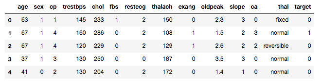  
![pandas load file][]

### 6.2.2 本地加载 ###

本地加载更加简单，应该所有学过机器学习的都接触过 pandas 的本地加载方法。

import pandas as pd
    
    csv_file = '/home/yan/.keras/datasets/heart.csv'
    df = pd.read_csv(csv_file)
    df.head()

![pandas load file][]

### 6.2.3 格式转换 ###

因为默认情况下 pandas读文件返回的是 pandas.core.frame.DataFrame 格式，需要进行格式转换。

import tensorflow as tf
    import pandas as pd
    
    csv_file = '/home/yan/.keras/datasets/heart.csv'
    df = pd.read_csv(csv_file)
    print(df.head())
    
    # 将这个属性格式 object 转换 int
    df['thal'] = pd.Categorical(df['thal'])
    df['thal'] = df.thal.cat.codes
    
    dataset = tf.data.Dataset.from_tensor_slices((df.values, target.values))
    dataset

输出内容为：

## 6.3 加载 numpy 数据集 ##

numpy 数据集一般以 `.npz` 为文件后缀，加载方法也非常简单，如例：

import numpy as np
    import tensorflow as tf
    
    DATA_URL = 'https://storage.googleapis.com/tensorflow/tf-keras-datasets/mnist.npz'
    
    path = tf.keras.utils.get_file('mnist.npz', DATA_URL)
    with np.load(path) as data:
        train_examples = data['x_train']
        train_labels = data['y_train']
        test_examples = data['x_test']
        test_labels = data['y_test']
        
    train_dataset = tf.data.Dataset.from_tensor_slices((train_examples, train_labels))
    test_dataset = tf.data.Dataset.from_tensor_slices((test_examples, test_labels))

## 6.4 加载图片 ##

加载图片数据集与上面提到的有很多不同之处，比如图片数据肯定是多个文件，而不是已经经过处理合并的单个文件，所以加载的时候需要一些处理技巧，甚至对于大图需要进行切割再逐个加载。

这里的例子是谷歌提供下载地址的多种花的 [图片][Link 5].

### 6.4.1 下载图片 ###

如果网速不好的话肯定需要几分钟时间，一般情况下1分钟内能够下载完成。

输出内容为：

PosixPath('/home/yan/.keras/datasets/flower_photos')

可以查看一下这个目录下的所有内容，里面包括内容如下：  
`daisy/ dandelion/ LICENSE.txt roses/ sunflowers/ tulips/`。

### 6.4.2 查看图片 ###

预处理前先查看一下数据，看看花儿。

import tensorflow as tf
    import PIL
    import pathlib
    dataset_url = "https://storage.googleapis.com/download.tensorflow.org/example_images/flower_photos.tgz"
    data_dir = tf.keras.utils.get_file(origin=dataset_url, 
                                       fname='flower_photos', 
                                       untar=True)
    data_dir = pathlib.Path(data_dir)
    
    roses = list(data_dir.glob('roses/*'))
    PIL.Image.open(str(roses[0]))

![在这里插入图片描述][watermark_type_ZmFuZ3poZW5naGVpdGk_shadow_10_text_aHR0cHM6Ly9ibG9nLmNzZG4ubmV0L3NtaWxleWFuOQ_size_16_color_FFFFFF_t_70_pic_center 2]

### 6.4.3 使用 tf.keras.preprocessing 加载数据 ###

过程非常简单，需要注意的是那些参数。

import tensorflow as tf
    import pathlib
    dataset_url = "https://storage.googleapis.com/download.tensorflow.org/example_images/flower_photos.tgz"
    data_dir = tf.keras.utils.get_file(origin=dataset_url, 
                                       fname='flower_photos', 
                                       untar=True)
    data_dir = pathlib.Path(data_dir)
    
    batch_size = 32
    img_height = 180
    img_width = 180
    
    train_ds = tf.keras.preprocessing.image_dataset_from_directory(
        data_dir,
        validation_split=0.2,
        subset="training",
        seed=123,
        image_size=(img_height, img_width),
        batch_size=batch_size)
    
    val_ds = tf.keras.preprocessing.image_dataset_from_directory(
      data_dir,
      validation_split=0.2,
      subset="validation",
      seed=123,
      image_size=(img_height, img_width),
      batch_size=batch_size)
    
    type(train_ds)

输出内容为：

Found 3670 files belonging to 5 classes.
    Using 2936 files for training.
    Found 3670 files belonging to 5 classes.
    Using 734 files for validation.
    <BatchDataset shapes: ((None, 180, 180, 3), (None,)), types: (tf.float32, tf.int32)>

这里只是加载图片简单例子，更多关于模型的训练与测试请参考 [官方文档][Link 6]

## 6.5 加载文本 ##

加载文本数据方法与图片差不多，需要注意参数的不同。

import tensorflow as tf
    import pathlib
    from tensorflow.keras import preprocessing
    
    from tensorflow.keras import utils
    
    data_url = 'https://storage.googleapis.com/download.tensorflow.org/data/stack_overflow_16k.tar.gz'
    
    data_dir = tf.keras.utils.get_file(origin=dataset_url, 
                                       fname='flower_photos', 
                                       untar=True)
    dataset = utils.get_file(
        'stack_overflow_16k.tar.gz',
        data_url,
        untar=True,
        cache_dir='stack_overflow',
        cache_subdir='')
    
    train_dir = dataset_dir/'train'
    # list(train_dir.iterdir())
    
    dataset_dir = pathlib.Path(dataset).parent
    
    batch_size = 32
    seed = 42
    
    raw_train_ds = preprocessing.text_dataset_from_directory(
        train_dir,
        batch_size=batch_size,
        validation_split=0.2,
        subset='training',
        seed=seed)
    
    raw_val_ds = preprocessing.text_dataset_from_directory(
        train_dir,
        batch_size=batch_size,
        validation_split=0.2,
        subset='validation',
        seed=seed)
    
    type(raw_train_ds)

输出内容为：

Found 8000 files belonging to 4 classes.
    Using 6400 files for training.
    Found 8000 files belonging to 4 classes.
    Using 1600 files for validation.
    tensorflow.python.data.ops.dataset_ops.BatchDataset

# 7. 总结 #

整理了一下学习笔记，不知不觉写了这么长（据 csdn 写博客网站统计约 3万字），总体上来说非常简单的 tensorflow2 的基础知识，希望能够写成字典式工具，当要用的时候在来这里看看，如果能找到就当复习一遍，如果不能找到就更新这篇博客。

当然，也希望能够帮助到其他在使用tensorflow2 遇到类似问题的人，如果觉得哪个地方表述不清楚或者有错误的话，请一定在后面评论，一定认真观看思考，感谢！

> Smileyan  
> 2020.10.25 21.02 发布  
> 2020.10.28 21:41 更新

[API]: https://tensorflow.google.cn/api_docs/python/tf
[Link 1]: https://search.bilibili.com/all?keyword=tensorflow2&from_source=nav_suggest_new
[Link 2]: https://github.com/dragen1860/Deep-Learning-with-TensorFlow-book
[Link 3]: https://study.163.com/course/introduction.htm?courseId=1209092816&_trace_c_p_k2_=aaf73e7e567049d989d3dc9fd973c0cb
[https_github.com_dragen1860_Deep-Learning-with-TensorFlow-book]: https://github.com/dragen1860/Deep-Learning-with-TensorFlow-book/blob/master/ch05-TensorFlow%E8%BF%9B%E9%98%B6/gradient_clip.py
[watermark_type_ZmFuZ3poZW5naGVpdGk_shadow_10_text_aHR0cHM6Ly9ibG9nLmNzZG4ubmV0L3NtaWxleWFuOQ_size_16_color_FFFFFF_t_70_pic_center]: /images/20221122/3aa6f08b96304865a5ff1432619a5406.png
[watermark_type_ZmFuZ3poZW5naGVpdGk_shadow_10_text_aHR0cHM6Ly9ibG9nLmNzZG4ubmV0L3NtaWxleWFuOQ_size_16_color_FFFFFF_t_70_pic_center 1]: /images/20221122/6f074f7ec62b442582484ed242b6b961.png
[boston_housing]: https://tensorflow.google.cn/api_docs/python/tf/keras/datasets/boston_housing
[mnist]: https://tensorflow.google.cn/api_docs/python/tf/keras/datasets/mnist
[fashion_mnist]: https://tensorflow.google.cn/api_docs/python/tf/keras/datasets/fashion_mnist
[cifar10]: https://tensorflow.google.cn/api_docs/python/tf/keras/datasets/cifar10
[cifar100]: https://tensorflow.google.cn/api_docs/python/tf/keras/datasets/cifar100?hl=en
[imdb]: https://tensorflow.google.cn/api_docs/python/tf/keras/datasets/imdb?hl=zh_cn
[reuters]: https://tensorflow.google.cn/api_docs/python/tf/keras/datasets/reuters?hl=zh_cn
[Link 4]: https://pandas.pydata.org/pandas-docs/stable/
[pandas load file]: /images/20221122/e22ed53f2d39499181dfe4dcf0f513e6.png
[Link 5]: https://storage.googleapis.com/download.tensorflow.org/example_images/flower_photos.tgz
[watermark_type_ZmFuZ3poZW5naGVpdGk_shadow_10_text_aHR0cHM6Ly9ibG9nLmNzZG4ubmV0L3NtaWxleWFuOQ_size_16_color_FFFFFF_t_70_pic_center 2]: /images/20221122/a646f82dc8064a59944564f81b76ec72.png
[Link 6]: https://tensorflow.google.cn/tutorials/load_data/images