PCA人脸识别
PCA方法由于其在降维和特征提取方面的有效性,在人脸识别领域得到了广泛的应用。
其基本原理是:利用K-L变换抽取人脸的主要成分,构成特征脸空间,识别时将测试图像投影到此空间,得到一组投影系数,通过与各个人脸图像比较进行识别。
进行人脸识别的过程,主要由训练阶段和识别阶段组成:
训练阶段
第一步:写出训练样本矩阵,其中向量xi为由第i个图像的每一列向量堆叠成一列的MN维列向量,即把矩阵向量化。假设训练集有200个样本,,由灰度图组成,每个样本大小为M*N。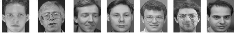
第二步:计算平均脸
Ψ=1200∑i=1i=200x**i
第三步:计算差值脸,计算每一张人脸与平均脸的差值
d**i=x**i−Ψ,i=1,2,…,200
第四步:构建协方差矩阵
C=1200∑i=1200didiT=1200AAT
第五步:求协方差矩阵的特征值和特征向量,构造特征脸空间
求出 ATA 的特征值 λ**i 及其正交归一化特征向量 ν**i ,根据特征值的贡献率选取前p个最大特征值及其对应的特征向量,贡献率是指选取的特征值的和与占所有特征值的和比,即:
ϕ=∑i=1i=pλi∑i=1i=200λ**i≥a
若选取前 p 个最大的特征值,则“特征脸”空间为:
w=(u1,u2,…u**p)
第六步:将每一幅人脸与平均脸的差值脸矢量投影到“特征脸”空间,即
Ωi=wTd**i(i=1,2,…,200)
识别阶段
第一步:将待识别的人脸图像Γ与平均脸的差值脸投影到特征脸空间,得到其特征向量表示:
ΩΓ=w**T(Γ−Ψ)
第二布:采用欧式距离来计算 ΩΓ 与每个人脸的距离 ε**i
ε**i2=∥∥Ωi−ΩΓ∥∥2(i=1,2,…,200)
求最小值对应的训练集合中的标签号作为识别结果
需要说明的是协方差矩阵 AAT 的维数为MN*MN,其维数是比较较大的,而我们在这里的训练样本个数为200, ATA 的维数为200*200小了许多,实际情况中,采用奇异值分解(SingularValue Decomposition ,SVD)定理,通过求解 ATA 的特征值和特征向量来组成特征脸空间的。必须明白的是特征脸空间是由 ATA 的子空间构成,我们的识别任务也是将原始 ATA 所构成的空间投影到我们选取前p个最大的特征值对应的特征向量组成的子空间里,进行比较,选取最近的训练样本为标号。
代码
训练过程代码如下:
function [m, A, Eigenfaces] = EigenfaceCore(T)% Use Principle Component Analysis (PCA) to determine the most% discriminating features between images of faces.%% Description: This function gets a 2D matrix, containing all training image vectors% and returns 3 outputs which are extracted from training database.%% Argument: T - A 2D matrix, containing all 1D image vectors.% Suppose all P images in the training database% have the same size of MxN. So the length of 1D% column vectors is M*N and 'T' will be a MNxP 2D matrix.%% Returns: m - (M*Nx1) Mean of the training database% Eigenfaces - (M*Nx(P-1)) Eigen vectors of the covariance matrix of the training database% A - (M*NxP) Matrix of centered image vectors%% See also: EIG% Original version by Amir Hossein Omidvarnia, October 2007% Email: aomidvar@ece.ut.ac.ir%%%%%%%%%%%%%%%%%%%%%%%% Calculating the mean imagem = mean(T,2); % Computing the average face image m = (1/P)*sum(Tj's) (j = 1 : P)Train_Number = size(T,2);%%%%%%%%%%%%%%%%%%%%%%%% Calculating the deviation of each image from mean imageA = [];for i = 1 : Train_Numbertemp = double(T(:,i)) - m; % Computing the difference image for each image in the training set Ai = Ti - mA = [A temp]; % Merging all centered imagesend%%%%%%%%%%%%%%%%%%%%%%%% Snapshot method of Eigenface methos% We know from linear algebra theory that for a PxQ matrix, the maximum% number of non-zero eigenvalues that the matrix can have is min(P-1,Q-1).% Since the number of training images (P) is usually less than the number% of pixels (M*N), the most non-zero eigenvalues that can be found are equal% to P-1. So we can calculate eigenvalues of A'*A (a PxP matrix) instead of% A*A' (a M*NxM*N matrix). It is clear that the dimensions of A*A' is much% larger that A'*A. So the dimensionality will decrease.L = A'*A; % L is the surrogate of covariance matrix C=A*A'.[V D] = eig(L); % Diagonal elements of D are the eigenvalues for both L=A'*A and C=A*A'.%%%%%%%%%%%%%%%%%%%%%%%% Sorting and eliminating eigenvalues% All eigenvalues of matrix L are sorted and those who are less than a% specified threshold, are eliminated. So the number of non-zero% eigenvectors may be less than (P-1).L_eig_vec = [];for i = 1 : size(V,2)if( D(i,i)>4e+07)L_eig_vec = [L_eig_vec V(:,i)];endend%%%%%%%%%%%%%%%%%%%%%%%% Calculating the eigenvectors of covariance matrix 'C'% Eigenvectors of covariance matrix C (or so-called "Eigenfaces")% can be recovered from L's eiegnvectors.Eigenfaces = A * L_eig_vec; % A: centered image vectors
识别过程代码如下:
function OutputName = Recognition(TestImage, m, A, Eigenfaces)% Recognizing step....%% Description: This function compares two faces by projecting the images into facespace and% measuring the Euclidean distance between them.%% Argument: TestImage - Path of the input test image%% m - (M*Nx1) Mean of the training% database, which is output of 'EigenfaceCore' function.%% Eigenfaces - (M*Nx(P-1)) Eigen vectors of the% covariance matrix of the training% database, which is output of 'EigenfaceCore' function.%% A - (M*NxP) Matrix of centered image% vectors, which is output of 'EigenfaceCore' function.%% Returns: OutputName - Name of the recognized image in the training database.%% See also: RESHAPE, STRCAT% Original version by Amir Hossein Omidvarnia, October 2007% Email: aomidvar@ece.ut.ac.ir%%%%%%%%%%%%%%%%%%%%%%%% Projecting centered image vectors into facespace% All centered images are projected into facespace by multiplying in% Eigenface basis's. Projected vector of each face will be its corresponding% feature vector.ProjectedImages = [];Train_Number = size(Eigenfaces,2);for i = 1 : Train_Numbertemp = Eigenfaces'*A(:,i); % Projection of centered images into facespaceProjectedImages = [ProjectedImages temp];end%%%%%%%%%%%%%%%%%%%%%%%% Extracting the PCA features from test imageInputImage = imread(TestImage);temp = InputImage(:,:,1);[irow icol] = size(temp);InImage = reshape(temp',irow*icol,1);Difference = double(InImage)-m; % Centered test imageProjectedTestImage = Eigenfaces'*Difference; % Test image feature vector%%%%%%%%%%%%%%%%%%%%%%%% Calculating Euclidean distances% Euclidean distances between the projected test image and the projection% of all centered training images are calculated. Test image is% supposed to have minimum distance with its corresponding image in the% training database.Euc_dist = [];for i = 1 : Train_Numberq = ProjectedImages(:,i);temp = ( norm( ProjectedTestImage - q ) )^2;Euc_dist = [Euc_dist temp];end[Euc_dist_min , Recognized_index] = min(Euc_dist);OutputName = strcat(int2str(Recognized_index),'.jpg');
其中训练样本的最后一行代码:
Eigenfaces = A * L_eig_vec; % A: centered image vectors
和识别过程的
temp = Eigenfaces'*A(:,i); % Projection of centered images into facespace
写成公式也就是如下
T=(A**V)T**A=V**T(ATA)
这里 V**T 是新坐标系下的基,投影的结果也就是新坐标系下的系数。基于PCA的人脸识别也就是我们在新的坐标系下比较两个向量的距离。完整代码下载地址点击 这里。
Licenses
| 作者 | 日期 | 联系方式 |
|---|---|---|
| 风吹夏天 | 2015年8月10日 | wincoder@qq.com |


拓扑排序")

")


还没有评论,来说两句吧...