Relation Networks for Object Detection(源码)
转自:https://blog.csdn.net/u014380165/article/details/80779712
论文:Relation Networks for Object Detection
论文链接:https://arxiv.org/abs/1711.11575
代码链接:https://github.com/msracver/Relation-Networks-for-Object-Detection
这篇文章的细节可以通过阅读源码来加深理解,这篇博客就来介绍这篇文章的部分源码。
因为这篇文章主要是在网络结构上做改动,所以这篇博客以resnet_v1_101_rcnn_attention_1024_pairwise_position_multi_head_16_learn_nms.py为例介绍网络结构,这个例子在Faster RCNN基础上引入relation module,包括全连接层和NMS阶段。
链接:resnet_v1_101_rcnn_attention_1024_pairwise_position_multi_head_16_learn_nms.py
接下来介绍的代码顺序和链接中的不大一样,这里按照代码运行时的顺序介绍,目的是方便跟着数据流进行阅读,主要涉及几个方法:全局网络构造:get_symbol;ROI信息的坐标变换:extract_position_matrix;ROI信息的坐标embedding:extract_position_embedding;object relation module的计算:attention_module_multi_head。
这里将网络结构封装成一个类,初始化函数中主要是resnet_v1_101网络的设置。
class resnet_v1_101_rcnn_attention_1024_pairwise_position_multi_head_16_learn_nms(resnet_v1_101_rcnn_learn_nms_base):def __init__(self):""" Use __init__ to define parameter network needs """self.eps = 1e-5self.use_global_stats = Trueself.workspace = 512self.units = (3, 4, 23, 3) # use for 101self.filter_list = [256, 512, 1024, 2048]
``
``
get_symbol方法是获取网络结构时候调用的方法,也是这个脚本中的主干,接下来都会围绕该方法进行介绍。在该方法中包含了整体网络结构的构造,非常重要。提取说明下,在ROI Pooling层之前的结构基本上和Faster RCNN类似,重点在于ROI Pooling层后面的两个全连接层。
def get_symbol(self, cfg, is_train=True):# config alias for convenient# 首先是一个参数设定。以COCO数据集为例(这篇文章的实验都是在COCO数据集上做的),# num_classes是81。cfg.CLASS_AGNOSTIC参数表示回归时是否不区分类别,默认是True,# 也就是不区分类别,因此num_reg_classes默认是2。需要注意的是原生的Faster RCNN在# 回归时是区分类别的。num_anchors默认是12,这个数值比原生的Faster RCNN要大。num_classes = cfg.dataset.NUM_CLASSESnum_reg_classes = (2 if cfg.CLASS_AGNOSTIC else num_classes)num_anchors = cfg.network.NUM_ANCHORS# input init# 输入数据和信息的初始化,需要和数据读取的变量同名。if is_train:data = mx.sym.Variable(name="data")im_info = mx.sym.Variable(name="im_info")gt_boxes = mx.sym.Variable(name="gt_boxes")rpn_label = mx.sym.Variable(name='label')rpn_bbox_target = mx.sym.Variable(name='bbox_target')rpn_bbox_weight = mx.sym.Variable(name='bbox_weight')else:data = mx.sym.Variable(name="data")im_info = mx.sym.Variable(name="im_info")# shared convolutional layers# conv_feat,包含resnet_v1_101从开始到conv4结束,这一部分是RPN网络的输入。# relu1,包含resnet_v1_101从开始到conv5结束,用来做object的坐标回归和分类。这都是常规的做法。conv_feat = self.get_resnet_v1_conv4(data)# res5relu1 = self.get_resnet_v1_conv5(conv_feat)# 这部分是基于conv_feat,调用get_rpn方法得到rpn网络的输出。rpn_cls_score, rpn_bbox_pred = self.get_rpn(conv_feat, num_anchors)if is_train:# prepare rpn datarpn_cls_score_reshape = mx.sym.Reshape(data=rpn_cls_score, shape=(0, 2, -1, 0), name="rpn_cls_score_reshape")# classification# 这部分是对bbox的二分类损失函数。rpn_cls_prob = mx.sym.SoftmaxOutput(data=rpn_cls_score_reshape, label=rpn_label, multi_output=True, normalization='valid', use_ignore=True, ignore_label=-1, name="rpn_cls_prob")# bounding box regression# 这部分是对bbox的坐标回归损失函数。rpn_bbox_loss_ = rpn_bbox_weight * mx.sym.smooth_l1(name='rpn_bbox_loss_', scalar=3.0, data=(rpn_bbox_pred - rpn_bbox_target))rpn_bbox_loss = mx.sym.MakeLoss(name='rpn_bbox_loss', data=rpn_bbox_loss_, grad_scale=1.0 / cfg.TRAIN.RPN_BATCH_SIZE)# ROI proposal# 这部分是对bbox做过滤得到proposal。注意几个参数:1、cfg.TRAIN.RPN_PRE_NMS_TOP_N表示# 进行NMS操作之前的roi数量,默认是6000。2、cfg.TRAIN.RPN_POST_NMS_TOP_N表示# NMS操作之后的roi操作,默认是300(FPN网络中默认用1000)。这两个参数设置和Faster RCNN不同。# 3、cfg.network.ANCHOR_SCALES默认是4,8,16,32。# 4、cfg.network.ANCHOR_RATIOS默认是0.5,1,2。rpn_cls_act = mx.sym.SoftmaxActivation(data=rpn_cls_score_reshape, mode="channel", name="rpn_cls_act")rpn_cls_act_reshape = mx.sym.Reshape(data=rpn_cls_act, shape=(0, 2 * num_anchors, -1, 0), name='rpn_cls_act_reshape')if cfg.TRAIN.CXX_PROPOSAL:rois = mx.contrib.sym.Proposal(cls_prob=rpn_cls_act_reshape, bbox_pred=rpn_bbox_pred, im_info=im_info, name='rois', feature_stride=cfg.network.RPN_FEAT_STRIDE, scales=tuple(cfg.network.ANCHOR_SCALES), ratios=tuple(cfg.network.ANCHOR_RATIOS), rpn_pre_nms_top_n=cfg.TRAIN.RPN_PRE_NMS_TOP_N, rpn_post_nms_top_n=cfg.TRAIN.RPN_POST_NMS_TOP_N, threshold=cfg.TRAIN.RPN_NMS_THRESH, rpn_min_size=cfg.TRAIN.RPN_MIN_SIZE)else:rois = mx.sym.Custom(cls_prob=rpn_cls_act_reshape, bbox_pred=rpn_bbox_pred, im_info=im_info, name='rois', op_type='proposal', feat_stride=cfg.network.RPN_FEAT_STRIDE,scales=tuple(cfg.network.ANCHOR_SCALES), ratios=tuple(cfg.network.ANCHOR_RATIOS),rpn_pre_nms_top_n=cfg.TRAIN.RPN_PRE_NMS_TOP_N, rpn_post_nms_top_n=cfg.TRAIN.RPN_POST_NMS_TOP_N, threshold=cfg.TRAIN.RPN_NMS_THRESH, rpn_min_size=cfg.TRAIN.RPN_MIN_SIZE)# ROI proposal target# 这部分一方面对前面的propsoal做过滤得到batch_rois个proposal(或者叫roi),最后# 得到的rois数量由cfg.TRAIN.BATCH_ROIS决定,这里因为cfg.TRAIN.BATCH_ROIS默认# 是-1(和Faster RCNN中默认的128不同),因此最后得到的roi数量等于输入roi的数量加# 上ground truth的数量,默认情况下输入roi数量是300,因此最后得到的roi数量是300+x,# x表示object的数量。另一方面计算Fast RCNN的分类和回归支路的训练目标。gt_boxes_reshape = mx.sym.Reshape(data=gt_boxes, shape=(-1, 5), name='gt_boxes_reshape')rois, label, bbox_target, bbox_weight = mx.sym.Custom(rois=rois, gt_boxes=gt_boxes_reshape, op_type='proposal_target', num_classes=num_reg_classes, batch_images=cfg.TRAIN.BATCH_IMAGES, batch_rois=cfg.TRAIN.BATCH_ROIS, cfg=cPickle.dumps(cfg),fg_fraction=cfg.TRAIN.FG_FRACTION)else:# 这部分是测试时候的网络结构设置,总体而言就是去掉了RPN网络的损失函数和Fast RCNN的# 分类和检测目标生成等。# ROI Proposalrpn_cls_score_reshape = mx.sym.Reshape(data=rpn_cls_score, shape=(0, 2, -1, 0), name="rpn_cls_score_reshape")rpn_cls_prob = mx.sym.SoftmaxActivation(data=rpn_cls_score_reshape, mode="channel", name="rpn_cls_prob")rpn_cls_prob_reshape = mx.sym.Reshape(data=rpn_cls_prob, shape=(0, 2 * num_anchors, -1, 0), name='rpn_cls_prob_reshape')if cfg.TEST.CXX_PROPOSAL:rois = mx.contrib.sym.Proposal(cls_prob=rpn_cls_prob_reshape, bbox_pred=rpn_bbox_pred, im_info=im_info, name='rois', feature_stride=cfg.network.RPN_FEAT_STRIDE, scales=tuple(cfg.network.ANCHOR_SCALES), ratios=tuple(cfg.network.ANCHOR_RATIOS),rpn_pre_nms_top_n=cfg.TEST.RPN_PRE_NMS_TOP_N, rpn_post_nms_top_n=cfg.TEST.RPN_POST_NMS_TOP_N,threshold=cfg.TEST.RPN_NMS_THRESH, rpn_min_size=cfg.TEST.RPN_MIN_SIZE)else:rois = mx.sym.Custom(cls_prob=rpn_cls_prob_reshape, bbox_pred=rpn_bbox_pred, im_info=im_info, name='rois', op_type='proposal', feat_stride=cfg.network.RPN_FEAT_STRIDE,scales=tuple(cfg.network.ANCHOR_SCALES), ratios=tuple(cfg.network.ANCHOR_RATIOS),rpn_pre_nms_top_n=cfg.TEST.RPN_PRE_NMS_TOP_N, rpn_post_nms_top_n=cfg.TEST.RPN_POST_NMS_TOP_N,threshold=cfg.TEST.RPN_NMS_THRESH, rpn_min_size=cfg.TEST.RPN_MIN_SIZE)# nongt_dim在训练中采用cfg.TRAIN.RPN_POST_NMS_TOP_N,默认是300,这个值在后续会经常用到。nongt_dim = cfg.TRAIN.RPN_POST_NMS_TOP_N if is_train else cfg.TEST.RPN_POST_NMS_TOP_N# 接下来这个卷积层是接在conv5后面的。conv_new_1 = mx.sym.Convolution(data=relu1, kernel=(1, 1), num_filter=256, name="conv_new_1")conv_new_1_relu = mx.sym.Activation(data=conv_new_1, act_type='relu', name='conv_new_1_relu')# ROIPooling是基于过滤得到的rois和前面计算的conv_new_1_relu计算得到,# 得到的roi_pool的维度是[num_rois, 256, 7, 7],这里的256是前面卷积层的卷积核数量。roi_pool = mx.symbol.ROIPooling(name='roi_pool', data=conv_new_1_relu, rois=rois, pooled_size=(7, 7), spatial_scale=0.0625)
``
``
以上内容和Faster RCNN基本上没有差别,真正有差别的地方在后面的两个全连接层,因为在这两个全连接层之间会引入这篇文章所说的object relation module。接下来就基于前面得到的roi进行坐标变换操作。
# 首先因为rois的维度1有5列,包含4个坐标值和1个index,因为后续只需要4个坐标值,# 所以这里做了slice操作得到sliced_rois。sliced_rois = mx.sym.slice_axis(rois, axis=1, begin=1, end=None)# [num_rois, nongt_dim, 4]# 这一步调用extract_position_matrix方法主要实现roi坐标的变换。position_matrix = self.extract_position_matrix(sliced_rois, nongt_dim=nongt_dim)
``
``
extract_position_matrix方法实现坐标的处理,对应论文中的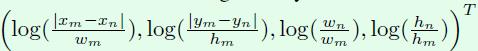
这里x、y、w和h分别表示中心点的横纵坐标、宽和高。接下来详细看看该方法的内容。
@staticmethoddef extract_position_matrix(bbox, nongt_dim):""" Extract position matrix Args: bbox: [num_boxes, 4] Returns: position_matrix: [num_boxes, nongt_dim, 4] """# xmin、ymin、xmax、ymax的维度都是[num_boxes, 1]xmin, ymin, xmax, ymax = mx.sym.split(data=bbox, num_outputs=4, axis=1)# [num_fg_classes, num_boxes, 1]# 根据xmin、ymin、xmax、ymax计算得到中心点坐标center_x、center_y,宽bbox_width和高bbox_heightbbox_width = xmax - xmin + 1.bbox_height = ymax - ymin + 1.center_x = 0.5 * (xmin + xmax)center_y = 0.5 * (ymin + ymax)# [num_fg_classes, num_boxes, num_boxes]# 执行broadcast_minus、broadcast_div后得到的delta_x的维度都是[num_boxes, num_boxes],# 且该矩阵的对角线都是0。执行log后得到的delta_x的维度仍然是[num_boxes, num_boxes],# 且对角线不存在0值,之所以log函数的输入有个maximum方法,是因为当log函数的输入是0时,输出是无穷小。delta_x = mx.sym.broadcast_minus(lhs=center_x,rhs=mx.sym.transpose(center_x))delta_x = mx.sym.broadcast_div(delta_x, bbox_width)delta_x = mx.sym.log(mx.sym.maximum(mx.sym.abs(delta_x), 1e-3))delta_y = mx.sym.broadcast_minus(lhs=center_y,rhs=mx.sym.transpose(center_y))delta_y = mx.sym.broadcast_div(delta_y, bbox_height)delta_y = mx.sym.log(mx.sym.maximum(mx.sym.abs(delta_y), 1e-3))delta_width = mx.sym.broadcast_div(lhs=bbox_width,rhs=mx.sym.transpose(bbox_width))delta_width = mx.sym.log(delta_width)delta_height = mx.sym.broadcast_div(lhs=bbox_height, rhs=mx.sym.transpose(bbox_height))delta_height = mx.sym.log(delta_height)# concat_list是一个长度为4的列表,列表中的每个值的维度是[num_boxes, num_boxes]。concat_list = [delta_x, delta_y, delta_width, delta_height]# 接下来这个循环会将concat_list列表中的每个值在维度1上取0到nongt_dim(默认是300),# 因此得到的sym的维度就是[num_boxes, nongt_dim];第二行则是新增了一个维度2,因此concat_list[idx]的# 维度就是[num_boxes, nongt_dim, 1]。因此最后得到的concat_list就是长度为4的列表,# 列表中的每个值的维度是[num_boxes, nongt_dim, 1],# concat后返回维度为[num_boxes, nongt_dim, 4]的position_matrix。for idx, sym in enumerate(concat_list):sym = mx.sym.slice_axis(sym, axis=1, begin=0, end=nongt_dim)concat_list[idx] = mx.sym.expand_dims(sym, axis=2)# 将concat_list列表中的4个值在维度2上进行concat,# 得到维度为[num_boxes, nongt_dim, 4]的position_matrix。position_matrix = mx.sym.concat(*concat_list, dim=2)return position_matrix
``
``
因此回到get_symbol方法,在得到position_matrix后,接下来就要做embedding了。
# [num_rois, nongt_dim, 64]# 这一步调用extract_position_embedding方法实现论文中公式5的EG操作。position_embedding = self.extract_position_embedding(position_matrix, feat_dim=64)
``
``
- 1
- 2
- 3
extract_position_embedding方法实现对geometry feature的embedding,具体而言就是实现论文中公式5中的这个操作。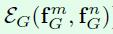
输入position_mat就是前面extract_position_matrix方法输出的position_matrix,也就是上面截图中的fG,m和n表示不同的roi,feat_dim默认采用64,接下来的维度都按照这个默认值来。接下来就来详细看看extract_position_embedding方法的内容。
@staticmethoddef extract_position_embedding(position_mat, feat_dim, wave_length=1000):# position_mat, [num_rois, nongt_dim, 4]# feat_range是[0,1,2,3,4,5,6,7]。full的第一个输入表示shape,第二个输入表示value,# 因此这里表示维度为1,值为1000的symbol。得到dim_mat=[1., 2.37137365, 5.62341309,# 13.33521461, 31.62277603, 74.98941803, 177.82794189, 421.69650269],# 维度是1*8,之后reshape成1*1*1*8。feat_range = mx.sym.arange(0, feat_dim / 8)dim_mat = mx.sym.broadcast_power(lhs=mx.sym.full((1,), wave_length), rhs=(8. / feat_dim) * feat_range)dim_mat = mx.sym.Reshape(dim_mat, shape=(1, 1, 1, -1))# position_mat增加维度3变成 [num_rois, nongt_dim, 4, 1],div_mat的维度# 是 [num_rois, nongt_dim, 4, 8],然后执行sin函数和cos函数操作得到相同维度的sin_mat和cos_mat。# 接着在维度3对sin_mat和cos_mat做concat操作,得到维度为[num_rois, nongt_dim, 4,# feat_dim/4]的输出,最后reshape成 [num_rois, nongt_dim, feat_dim]的embedding。position_mat = mx.sym.expand_dims(100.0 * position_mat, axis=3)div_mat = mx.sym.broadcast_div(lhs=position_mat, rhs=dim_mat)sin_mat = mx.sym.sin(data=div_mat)cos_mat = mx.sym.cos(data=div_mat)# embedding, [num_rois, nongt_dim, 4, feat_dim/4]embedding = mx.sym.concat(sin_mat, cos_mat, dim=3)# embedding, [num_rois, nongt_dim, feat_dim]embedding = mx.sym.Reshape(embedding, shape=(0, 0, feat_dim))return embedding
``
``
再回到get_symbol方法,做完坐标信息的embedding后,接下来就是重头戏了。
# 2 fc# 首先是常规的全连接层,得到的fc_new_1的维度是[num_rois, 1024]。fc_new_1 = mx.symbol.FullyConnected(name='fc_new_1', data=roi_pool, num_hidden=1024)# attention, [num_rois, feat_dim]# 这一步调用attention_module_multi_head方法,按顺序实现论文中公式5、4、3、2的内容# 和公式6的后半部分内容,因此基本上包含了论文的核心。得到的attention_1(维度为[num_rois, 1024],# 这个1024和前面的全连接层参数对应)就是论文中公式6的concat部分内容,# 而公式6的加法部分通过 fc_all_1 = fc_new_1 + attention_1得到。attention_1 = self.attention_module_multi_head(fc_new_1, position_embedding, nongt_dim=nongt_dim, fc_dim=16, feat_dim=1024, index=1, group=16, dim=(1024, 1024, 1024))
``
``
因为attention_module_embedding方法是这篇文章大部分公式的实现,因此来详细看下源码。
# roi_feat: [num_rois, feat_dim],这里的feat_dim默认是1024,对应前面全连接层的维度,# 因此和 extract_position_embedding方法中的feat_dim不是一回事,# extract_position_embedding方法的输出对应这里的输入position_embedding,维度# 是[num_rois, nongt_dim, emb_dim],注意emb_dim和feat_dim的区别。fc_dim要和group相等。def attention_module_multi_head(self, roi_feat, position_embedding, nongt_dim, fc_dim, feat_dim, dim=(1024, 1024, 1024), group=16, index=1):""" Attetion module with vectorized version Args: roi_feat: [num_rois, feat_dim] position_embedding: [num_rois, nongt_dim, emb_dim] nongt_dim: fc_dim: should be same as group feat_dim: dimension of roi_feat, should be same as dim[2] dim: a 3-tuple of (query, key, output) group: index: Returns: output: [num_rois, ovr_feat_dim, output_dim] """# 因为dim默认是(1024, 1024, 1024),group默认是16,所以dim_group就是(64, 64, 64)。# 然后在roi_feat的维度0上选取前nongt_dim的值,得到的nongt_roi_feat的维度是[nongt_dim, feat_dim]。dim_group = (dim[0] / group, dim[1] / group, dim[2] / group)nongt_roi_feat = mx.symbol.slice_axis(data=roi_feat, axis=0, begin=0, end=nongt_dim)# [num_rois * nongt_dim, emb_dim]# 调用reshape方法将维度为[num_rois, nongt_dim, emb_dim]的position_embedding reshape成# [num_rois*nongt_dim, emb_dim]的position_embedding_reshape。position_embedding_reshape = mx.sym.Reshape(position_embedding, shape=(-3, -2))# position_feat_1, [num_rois * nongt_dim, fc_dim]# 用全连接层实现论文中公式5的max函数输入,全连接层的参数就是公式5的WG。输入是预测框位置信息# 的embedding结果:position_embedding_reshape,得到维度为[num_rois * nongt_dim, fc_dim]# 的position_feat_1。然后reshape成维度为[num_rois, nongt_dim, fc_dim]的aff_weight,# 最后调换维度得到维度为 [num_rois, fc_dim, nongt_dim] 的aff_weight。position_feat_1 = mx.sym.FullyConnected(name='pair_pos_fc1_' + str(index), data=position_embedding_reshape, num_hidden=fc_dim)position_feat_1_relu = mx.sym.Activation(data=position_feat_1, act_type='relu')# aff_weight, [num_rois, nongt_dim, fc_dim]aff_weight = mx.sym.Reshape(position_feat_1_relu, shape=(-1, nongt_dim, fc_dim))# aff_weight, [num_rois, fc_dim, nongt_dim]aff_weight = mx.sym.transpose(aff_weight, axes=(0, 2, 1))# multi head# 用全连接层得到q_data,全连接层参数对应论文中公式4的WQ,roi_feat对应公式4的fA,维度# 是[num_rois, feat_dim]。reshape后得到的q_data_batch维度是[num_rois, group, dim_group[0]],# 默认是[num_rois, 16, 64],transpose后得到的q_data_batch维度# 是[group, num_rois, dim_group[0]],默认是[16, num_rois, 64]。assert dim[0] == dim[1], 'Matrix multiply requires same dimensions!'q_data = mx.sym.FullyConnected(name='query_' + str(index),data=roi_feat,num_hidden=dim[0])q_data_batch = mx.sym.Reshape(q_data, shape=(-1, group, dim_group[0]))q_data_batch = mx.sym.transpose(q_data_batch, axes=(1, 0, 2))# 用全连接层得到k_data,全连接层参数对应论文中公式4的WK,nongt_roi_feat对应公式4中的fA,# 维度是[nongt_dim, feat_dim],最后经过reshape和transpose后得到的k_data_batch# 的维度是[group, nongt_dim, dim_group[0]],默认是[16, nongt_dim, 64]。k_data = mx.symbol.FullyConnected(name='key_' + str(index),data=nongt_roi_feat,num_hidden=dim[1])k_data_batch = mx.sym.Reshape(k_data, shape=(-1, group, dim_group[1]))k_data_batch = mx.sym.transpose(k_data_batch, axes=(1, 0, 2))v_data = nongt_roi_feat# v_data = mx.symbol.FullyConnected(name='value_'+str(index)+'_'+str(gid), data=roi_feat, num_hidden=dim_group[2])# 这个batch_dot操作就是论文中公式4的dot,dot就是矩阵乘法。# 得到的aff维度是[group, num_rois, nongt_dim],默认是[16, num_rois, nongt_dim]。# 然后做一个scale操作,对应论文中公式4的除法。最后transpose得到维度为# [num_rois, group, nongt_dim]的aff_scale。这个aff_scale就是论文中公式4的结果:wA。aff = mx.symbol.batch_dot(lhs=q_data_batch, rhs=k_data_batch, transpose_a=False, transpose_b=True)# aff_scale, [group, num_rois, nongt_dim]aff_scale = (1.0 / math.sqrt(float(dim_group[1]))) * affaff_scale = mx.sym.transpose(aff_scale, axes=(1, 0, 2))assert fc_dim == group, 'fc_dim != group'# weighted_aff, [num_rois, fc_dim, nongt_dim]# aff_scale表示wA,前面的log函数输入:mx.sym.maximum(left=aff_weight, right=1e-6)# 对应论文中公式5,之所以要求log,是因为这里要用softmax实现论文3的公式,而在softmax中# 会对输入求指数(以e为底),而要达到论文中公式3的形式(e的指数只有wA,没有wG),# 就要先对wGmn求log,这样再求指数时候就恢复成wG。简而言之就是e^(log(wG)+wA)=wG+e^(wA)。# softmax实现论文中公式3的操作,axis设置为2表示在维度2上进行归一化。# 最后对维度为[num_rois, fc_dim, nongt_dim]的aff_softmax做reshape操作得到维度# 为[num_rois * fc_dim, nongt_dim]的aff_softmax_reshape,# aff_softmax_reshape也就对应论文中公式3的w。weighted_aff = mx.sym.log(mx.sym.maximum(left=aff_weight, right=1e-6)) + aff_scaleaff_softmax = mx.symbol.softmax(data=weighted_aff, axis=2, name='softmax_' + str(index))# [num_rois * fc_dim, nongt_dim]aff_softmax_reshape = mx.sym.Reshape(aff_softmax, shape=(-3, -2))# output_t, [num_rois * fc_dim, feat_dim]# dot函数的输入aff_softmax_reshape维度是[num_rois * fc_dim, nongt_dim],# v_data的维度是[nongt_dim, feat_dim],因此得到的output_t的维度# 是[num_rois * fc_dim, feat_dim],对应论文中公式2的w和fA相乘的结果。# reshape后得到维度为[num_rois, fc_dim*feat_dim,1,1]的output_t。output_t = mx.symbol.dot(lhs=aff_softmax_reshape, rhs=v_data)# output_t, [num_rois, fc_dim * feat_dim, 1, 1]output_t = mx.sym.Reshape(output_t, shape=(-1, fc_dim * feat_dim, 1, 1))# linear_out, [num_rois, dim[2], 1, 1]# 最后用卷积核数量为dim[2](默认是1024)的1*1卷积得到维度为[num_rois, dim[2], 1, 1]的lineae_out,# 卷积层的参数对应论文中公式2的WV,reshape后得到维度为[num_rois, dim[2]]的output,# 这样得到的linear_out就是论文中公式2的fR。注意这里的卷积层有个num_group参数,# group数量设置为fc_dim,默认是16,对应论文中的Nr参数,因此论文中公式6的concat操# 作已经在这个卷积层中通过group操作实现了。linear_out = mx.symbol.Convolution(name='linear_out_' + str(index), data=output_t, kernel=(1, 1), num_filter=dim[2], num_group=fc_dim)output = mx.sym.Reshape(linear_out, shape=(0, 0))return output
``
``
再回到get_symbol方法,前面attention_module_multi_head方法的目的就是得到attention_1,这个就是文章中提到的relation特征。接下来就是特征融合操作了。
# attention特征和原来的全连接层输出特征融合fc_all_1 = fc_new_1 + attention_1fc_all_1_relu = mx.sym.Activation(data=fc_all_1, act_type='relu', name='fc_all_1_relu')# 对fc_new_2同样调用了attention_module_multi_head方法得到attention_2,然后得到fc_all_2fc_new_2 = mx.symbol.FullyConnected(name='fc_new_2', data=fc_all_1_relu, num_hidden=1024)attention_2 = self.attention_module_multi_head(fc_new_2, position_embedding,nongt_dim=nongt_dim, fc_dim=16, feat_dim=1024, index=2, group=16, dim=(1024, 1024, 1024))fc_all_2 = fc_new_2 + attention_2fc_all_2_relu = mx.sym.Activation(data=fc_all_2, act_type='relu', name='fc_all_2_relu')# cls_score/bbox_pred# 接下来基于添加了attention的特征进行回归和分类。这里要注意的是在原生的Faster RCNN算法中,# 对proposal的回归是区别类别的,比如对于COCO数据集而言,一共包含80个object类,# 回归的全连接层的num_hidden参数是4*(80+1),而这里采用的是不区别类别的回归,# 因此num_reg_classes是2而不是类似COCO数据集中的81。另外在SSD算法中,# 回归支路用卷积层实现时卷积核的数量是num_anchors*4,和这里也不大一样。cls_score = mx.symbol.FullyConnected(name='cls_score', data=fc_all_2_relu, num_hidden=num_classes)bbox_pred = mx.symbol.FullyConnected(name='bbox_pred', data=fc_all_2_relu, num_hidden=num_reg_classes * 4)if is_train:# 如果有用到ohem算法,则通过自定义层得到ohem算法的权重和标签。if cfg.TRAIN.ENABLE_OHEM:labels_ohem, bbox_weights_ohem = mx.sym.Custom(op_type='BoxAnnotatorOHEM', num_classes=num_classes, num_reg_classes=num_reg_classes, roi_per_img=cfg.TRAIN.BATCH_ROIS_OHEM, cls_score=cls_score, bbox_pred=bbox_pred, labels=label, bbox_targets=bbox_target, bbox_weights=bbox_weight)# 分类部分采用softmaxout层实现,回归用smooth_l1层实现,这二者和Faster RCNN是一样的。# 只不过引入ohem的话,主要的不同点在于分类时候的标签用的是labels_ohem,# 回归时候的weight用的是bbox_weights_ohem。cls_prob = mx.sym.SoftmaxOutput(name='cls_prob', data=cls_score, label=labels_ohem, normalization='valid', use_ignore=True, ignore_label=-1)bbox_loss_ = bbox_weights_ohem * mx.sym.smooth_l1(name='bbox_loss_', scalar=1.0, data=(bbox_pred - bbox_target))bbox_loss = mx.sym.MakeLoss(name='bbox_loss', data=bbox_loss_, grad_scale=1.0 / cfg.TRAIN.BATCH_ROIS_OHEM)rcnn_label = labels_ohemelse:cls_prob = mx.sym.SoftmaxOutput(name='cls_prob', data=cls_score, label=label, normalization='valid')bbox_loss_ = bbox_weight * mx.sym.smooth_l1(name='bbox_loss_', scalar=1.0, data=(bbox_pred - bbox_target))if cfg.TRAIN.BATCH_ROIS < 0:batch_rois_num = 300else:batch_rois_num = cfg.TRAIN.BATCH_ROISbbox_loss = mx.sym.MakeLoss(name='bbox_loss', data=bbox_loss_, grad_scale=1.0 / batch_rois_num)rcnn_label = label# reshape output# 最后就是一些reshape操作和最终的group操作rcnn_label = mx.sym.Reshape(data=rcnn_label, shape=(cfg.TRAIN.BATCH_IMAGES, -1), name='label_reshape')cls_prob = mx.sym.Reshape(data=cls_prob, shape=(cfg.TRAIN.BATCH_IMAGES, -1, num_classes), name='cls_prob_reshape')bbox_loss = mx.sym.Reshape(data=bbox_loss, shape=(cfg.TRAIN.BATCH_IMAGES, -1, 4 * num_reg_classes), name='bbox_loss_reshape')output_sym_list = [rpn_cls_prob, rpn_bbox_loss, cls_prob, bbox_loss, mx.sym.BlockGrad(rcnn_label)]# 这个else语句是在测试时候进行的,此时就不需要计算损失函数else:cls_prob = mx.sym.SoftmaxActivation(name='cls_prob', data=cls_score)cls_prob = mx.sym.Reshape(data=cls_prob, shape=(cfg.TEST.BATCH_IMAGES, -1, num_classes), name='cls_prob_reshape')bbox_pred_reshape = mx.sym.Reshape(data=bbox_pred, name='bbox_pred_reshape', shape=(cfg.TEST.BATCH_IMAGES, -1, 4 * num_reg_classes))output_sym_list = [rois, cls_prob, bbox_pred_reshape]if is_train and (not cfg.TRAIN.LEARN_NMS):raise ValueError('config.TRAIN.LEARN_NMS is set to false!')elif (not is_train) and (not cfg.TEST.LEARN_NMS):self.sym = mx.sym.Group(output_sym_list)# print self.sym.list_outputs()return self.sym
``
``
接下来这部分是论文中在nms过程插入object relation module的过程,同样是在get_symbol方法中实现的。
######################### learn nms ########################## notice that all implementation of python ops try to leave batch idx support for multi-batch# thus, rois are [batch_ind, x_min, y_min, x_max, y_max]# 首先是一个参数设置信息:cfg.network.NMS_TARGET_THRESH默认采用'0.5, 0.6, 0.7, 0.8, 0.9'。# cfg.TRAIN.FIRST_N默认是100。cfg.TRAIN.BBOX_MEANS默认是0.0, 0.0, 0.0, 0.0,# cfg.TRAIN.BBOX_STDS默认是0.1, 0.1, 0.2, 0.2,cfg.RPN_POST_NMS_TOP_N默认是300 。# num_fg_classes参数是不包含背景的类别数,也就是object的类别数量。nms_target_thresh = np.fromstring(cfg.network.NMS_TARGET_THRESH, dtype=float, sep=',')num_thresh = len(nms_target_thresh)nms_eps = 1e-8first_n = cfg.TRAIN.FIRST_N if is_train else cfg.TEST.FIRST_Nnum_fg_classes = num_classes - 1bbox_means = cfg.TRAIN.BBOX_MEANS if is_train else Nonebbox_stds = cfg.TRAIN.BBOX_STDS if is_train else Nonenongt_dim = cfg.TRAIN.RPN_POST_NMS_TOP_N if is_train else cfg.TEST.RPN_POST_NMS_TOP_N# 整体上也是区分训练和测试阶段。if is_train:# remove gt here# cls_score是分类支路的输出,维度是[num_rois, num_classes];bbox_pred是回归支路的输出,# 维度是[num_rois, num_reg_classes*4],这里都在维度0上截取前nongt_dim个roi。cls_score_nongt = mx.sym.slice_axis(data=cls_score, axis=0, begin=0, end=nongt_dim)bbox_pred_nongt = mx.sym.slice_axis(data=bbox_pred, axis=0, begin=0, end=nongt_dim)bbox_pred_nongt = mx.sym.BlockGrad(bbox_pred_nongt)# refine bbox# remove batch idx and gt roi# 这里对原本维度为[num_rois, 5]的rois执行slice操作,得到维度为[nongt_dim,4]的sliced_rois。sliced_rois = mx.sym.slice(data=rois, begin=(0, 1), end=(nongt_dim, None))# bbox_pred_nobg, [num_rois, 4*(num_reg_classes-1)]# bbox_pred_nobg是forground的回归值,维度是[nongt_dim, 4]bbox_pred_nobg = mx.sym.slice_axis(data=bbox_pred_nongt, axis=1, begin=4, end=None)# [num_boxes, 4, num_reg_classes-1]# refine_bbox是基类resnet_v1_101_rcnn_learn_nms_base的方法,输入sliced_rois是roi的4个坐标信息,# bbox_pred_nobg是回归得到的坐标offset,因此这个方法就是根据这两个输入,# 按照Faster RCNN算法中公式2(参考最后附录中的截图)计算出预测框的# 真实坐标(xmin/ymin/xmax/ymax,而不是offset),refined_bbox的维度是[nongt_dim,4]。refined_bbox = self.refine_bbox(sliced_rois, bbox_pred_nobg, im_info, means=bbox_means, stds=bbox_stds)# softmax cls_score to cls_prob, [num_rois, num_classes]# 对维度为[nongt_dim, num_classes]的cls_score_nongt的最后一个维度进行softmax计算。# 然后对cls_prob在维度1上截取从1到最后的值,得到的cls_prob_nobg表示object分类的结果,# 维度是[nongt_dim, num_fg_classes]。cls_prob = mx.sym.softmax(data=cls_score_nongt, axis=-1)cls_prob_nobg = mx.sym.slice_axis(cls_prob, axis=1, begin=1, end=None)# 接下来对cls_prob_nobg在维度0上进行排序(is_ascend=False表示降序),# 也就是对每一列的数值都按照降序排列,什么意思呢?举个例子,# 假设待排序的数组(cls_prob_nobg)是# [[0.17, 0.22, 0.87, 0.92, 0.67],[0.75, 0.96, 0.55, 0.56, 0.36],[0.47, 0.06, 0.3, 0.18, 0.66]],# 那么排序后(sorted_cls_prob_nobg)就是# [[0.75, 0.96, 0.87, 0.92, 0.67],[0.47, 0.22, 0.55, 0.56, 0.66],[0.17, 0.06, 0.3, 0.18, 0.36]]。# 最后再截取概率最高的前first_n个roi,first_n默认是100。因此从排序结果就可以得到针对每个类别,# 预测概率从高到低的排序结果。sorted_cls_prob_nobg = mx.sym.sort(data=cls_prob_nobg, axis=0, is_ascend=False)# sorted_score, [first_n, num_fg_classes]sorted_score = mx.sym.slice_axis(sorted_cls_prob_nobg, axis=0, begin=0, end=first_n, name='sorted_score')# sort by score# 这里同样是在维度0上对cls_prob_nobg进行排序(降序),但这里得到的是index,这样就# 能够知道对每个类别而言,每个roi的预测概率排序结果。还是以前面那个排序数组为例,# 则得到的rank_indices就是[[1,1,0,0,0],[2,0,1,1,2],[0,2,2,2,1]],# 所以对类别0而言,roi 1的概率最高,其次是roi 2,最后时roi 0。# 同样最后再截取前first_n个roi,first_n默认是100。rank_indices = mx.sym.argsort(data=cls_prob_nobg, axis=0, is_ascend=False)# first_rank_indices, [first_n, num_fg_classes]first_rank_indices = mx.sym.slice_axis(rank_indices, axis=0, begin=0, end=first_n)# sorted_bbox, [first_n, num_fg_classes, 4, num_reg_classes-1]# take操作是根据first_rank_indices从refined_bbox中取数的过程,# first_rank_indices的维度是[first_n, num_fg_classes],refined_bbox的维度是[nongt_dim, 4],# 而得到的sorted_bbox变量的维度是[first_n, num_fg_classes, 4],这是因为first_rank_indices# 变量里面的值就是refined_bbox中的行index。因此sorted_bbox这个3维矩阵的含义是对# 于每个类别而言(维度1),roi的预测概率最高的前first_n个roi(维度0)的4个坐标信息(维度2)。sorted_bbox = mx.sym.take(a=refined_bbox, indices=first_rank_indices)# 因为cfg.CLASS_AGNOSTIC默认是true且sorted_bbox是3维的,所以sorted_bbox不变。if cfg.CLASS_AGNOSTIC:# sorted_bbox, [first_n, num_fg_classes, 4]sorted_bbox = mx.sym.Reshape(sorted_bbox, shape=(0, 0, 0), name='sorted_bbox')else:cls_mask = mx.sym.arange(0, num_fg_classes)cls_mask = mx.sym.Reshape(cls_mask, shape=(1, -1, 1))cls_mask = mx.sym.broadcast_to(cls_mask, shape=(first_n, 0, 4))# sorted_bbox, [first_n, num_fg_classes, 4]sorted_bbox = mx.sym.pick(data=sorted_bbox, name='sorted_bbox', index=cls_mask, axis=3)# nms_rank_embedding, [first_n, 1024]# extract_rank_embedding方法是基类resnet_v1_101_rcnn_learn_nms_base的方法,# 做法类似前面介绍的extract_position_embedding方法,得到的nms_rank_embedding维度是[first_n, 1024]。# 然后接一个num_hidden=128的全连接层,得到维度为[first_n ,128]的nms_rank_feat。nms_rank_embedding = self.extract_rank_embedding(first_n, 1024)# nms_rank_feat, [first_n, 1024]nms_rank_feat = mx.sym.FullyConnected(name='nms_rank', data=nms_rank_embedding, num_hidden=128)# nms_position_matrix, [num_fg_classes, first_n, first_n, 4]# extract_multi_position_matrix方法是基类resnet_v1_101_rcnn_learn_nms_base的方法,# 输入是维度为[first_n, num_fg_classes, 4]的sorted_bbox。该方式实现的内容和前# 面介绍的extract_position_matrix方法类似,可以简单概括为实现论文中的那个坐标变换,# 得到的nms_position_matrix维度是[num_fg_classes, first_n, first_n, 4]。nms_position_matrix = self.extract_multi_position_matrix(sorted_bbox)# roi_feature_embedding, [num_rois, 1024]# 这个全连接层的输入是fc_all_2_relu(维度为[num_rois, 1024]),这个变量是整个检# 测算法最终提取到的特征,该特征包含了这篇文章中的object relation module的结果,# 而且最后的坐标回归和分类都是直接基于这个特征进行的。因此这里的全连接层作用还是特征的embedding,# 得到的roi_feat_embedding维度是[num_rois, 128]。最后接一个take操作,这个前面已经介绍过了,# 就是从roi_feat_embedding中抽取指定index(first_rank_indices)的过程,# 最后得到维度为[first_n, num_fg_classes, 128]的sorted_roi_feat。# 因此sorted_roi_feat这个3维矩阵的含义是对于每个类别而言(维度1),# roi的预测概率最高的前first_n个roi(维度0)的128维特征信息(维度2)。roi_feat_embedding = mx.sym.FullyConnected(name='roi_feat_embedding',data=fc_all_2_relu,num_hidden=128)# sorted_roi_feat, [first_n, num_fg_classes, 128]sorted_roi_feat = mx.sym.take(a=roi_feat_embedding, indices=first_rank_indices)# vectorized nms# nms_embedding_feat, [first_n, num_fg_classes, 128]# mx.sym.expand_dims(nms_rank_feat, axis=1)操作将维度为[first_n ,128]的nms_rank_feat# 扩充为[first_n, 1, 128],然后和维度为[first_n. num_fg_classes, 128]的sorted_roi_feat# 做加法得到维度为[first_n. num_fg_classes, 128]的nms_embedding_feat。nms_embedding_feat = mx.sym.broadcast_add(lhs=sorted_roi_feat,rhs=mx.sym.expand_dims(nms_rank_feat, axis=1))# nms_attention_1, [first_n, num_fg_classes, 1024]# attention_module_nms_multi_head方法和前面提到的attention_module_multi_head# 方法类似,都是完成论文中几个公式。nms_attention_1, nms_softmax_1 = self.attention_module_nms_multi_head(nms_embedding_feat, nms_position_matrix,num_rois=first_n, index=1, group=16,dim=(1024, 1024, 128), fc_dim=(64, 16), feat_dim=128)# 将原来的embedding特征和attention特征融合得到nms_all_feat_1,# 维度仍然是[first_n, num_fg_classes, 128]。然后reshape成维度为[first_n*num_fg_classes, 128]# 的nms_all_feat_1_relu_reshape。再接一个num_hidden=num_thresh的全连接层,num_thresh默认是5,# 因此得到维度为[first_n * num_fg_classes, num_thresh]的nms_conditional_logit。# 再将nms_conditional_logit转换成维度为[first_n, num_fg_classes, num_thresh]的# nms_conditional_logit_reshape,然后用sigmod激活函数进行激活得到维度# 为[first_n, num_fg_classes, num_thresh]的nms_conditional_score。nms_all_feat_1 = nms_embedding_feat + nms_attention_1nms_all_feat_1_relu = mx.sym.Activation(data=nms_all_feat_1, act_type='relu', name='nms_all_feat_1_relu')# [first_n * num_fg_classes, 1024]nms_all_feat_1_relu_reshape = mx.sym.Reshape(nms_all_feat_1_relu, shape=(-3, -2))# logit, [first_n * num_fg_classes, num_thresh]nms_conditional_logit = mx.sym.FullyConnected(name='nms_logit', data=nms_all_feat_1_relu_reshape, num_hidden=num_thresh)# logit_reshape, [first_n, num_fg_classes, num_thresh]nms_conditional_logit_reshape = mx.sym.Reshape(nms_conditional_logit, shape=(first_n, num_fg_classes, num_thresh))nms_conditional_score = mx.sym.Activation(data=nms_conditional_logit_reshape, act_type='sigmoid', name='nms_conditional_score')# 这里对维度为[first_n, num_fg_classes]的sorted_score增加维度2,并和维度# 为[first_n, num_fg_classes, num_thresh]的nms_conditional_score相乘得到# 维度为[first_n, num_fg_classes, num_thresh]的nms_multi_score。sorted_score_reshape = mx.sym.expand_dims(sorted_score, axis=2)# sorted_score_reshape = mx.sym.BlockGrad(sorted_score_reshape)nms_multi_score = mx.sym.broadcast_mul(lhs=sorted_score_reshape, rhs=nms_conditional_score)# else是测试时候的条件语句,和前面训练部分的代码差别较大,这里主要通过一个自定义层来实现nms操作。else:nms_rank_weight = mx.sym.var('nms_rank_weight', shape=(128, 1024), dtype=np.float32)nms_rank_bias = mx.sym.var('nms_rank_bias', shape=(128,), dtype=np.float32)roi_feat_embedding_weight = mx.sym.var('roi_feat_embedding_weight', shape=(128, 1024), dtype=np.float32)roi_feat_embedding_bias = mx.sym.var('roi_feat_embedding_bias', shape=(128,), dtype=np.float32)nms_pair_pos_fc1_1_weight = mx.sym.var('nms_pair_pos_fc1_1_weight', shape=(16, 64), dtype=np.float32)nms_pair_pos_fc1_1_bias = mx.sym.var('nms_pair_pos_fc1_1_bias', shape=(16,), dtype=np.float32)nms_query_1_weight = mx.sym.var('nms_query_1_weight', shape=(1024, 128), dtype=np.float32)nms_query_1_bias = mx.sym.var('nms_query_1_bias', shape=(1024,), dtype=np.float32)nms_key_1_weight = mx.sym.var('nms_key_1_weight', shape=(1024, 128), dtype=np.float32)nms_key_1_bias = mx.sym.var('nms_key_1_bias', shape=(1024,), dtype=np.float32)nms_linear_out_1_weight = mx.sym.var('nms_linear_out_1_weight', shape=(128, 128, 1, 1), dtype=np.float32)nms_linear_out_1_bias = mx.sym.var('nms_linear_out_1_bias', shape=(128,), dtype=np.float32)nms_logit_weight = mx.sym.var('nms_logit_weight', shape=(5, 128), dtype=np.float32)nms_logit_bias = mx.sym.var('nms_logit_bias', shape=(5,), dtype=np.float32)nms_multi_score, sorted_bbox, sorted_score = mx.sym.Custom(cls_score=cls_score, bbox_pred=bbox_pred, rois=rois, im_info=im_info, nms_rank_weight=nms_rank_weight, fc_all_2_relu=fc_all_2_relu, nms_rank_bias=nms_rank_bias, roi_feat_embedding_weight=roi_feat_embedding_weight, roi_feat_embedding_bias= roi_feat_embedding_bias, nms_pair_pos_fc1_1_weight=nms_pair_pos_fc1_1_weight, nms_pair_pos_fc1_1_bias=nms_pair_pos_fc1_1_bias, nms_query_1_weight=nms_query_1_weight, nms_query_1_bias=nms_query_1_bias,nms_key_1_weight=nms_key_1_weight, nms_key_1_bias=nms_key_1_bias,nms_linear_out_1_weight= nms_linear_out_1_weight,nms_linear_out_1_bias=nms_linear_out_1_bias,nms_logit_weight=nms_logit_weight, nms_logit_bias=nms_logit_bias,op_type='learn_nms', name='learn_nms', num_fg_classes=num_fg_classes,bbox_means=bbox_means, bbox_stds=bbox_stds, first_n=first_n,class_agnostic=cfg.CLASS_AGNOSTIC, num_thresh=num_thresh,class_thresh=cfg.TEST.LEARN_NMS_CLASS_SCORE_TH, nongt_dim=nongt_dim, has_non_gt_index=False)if is_train:nms_multi_target = mx.sym.Custom(bbox=sorted_bbox, gt_bbox=gt_boxes, score=sorted_score, op_type='nms_multi_target', target_thresh=nms_target_thresh)nms_pos_loss = - mx.sym.broadcast_mul(lhs=nms_multi_target, rhs=mx.sym.log(data=(nms_multi_score + nms_eps)))nms_neg_loss = - mx.sym.broadcast_mul(lhs=(1.0 - nms_multi_target), rhs=mx.sym.log(data=(1.0 - nms_multi_score + nms_eps)))normalizer = first_n * num_threshnms_pos_loss = cfg.TRAIN.nms_loss_scale * nms_pos_loss / normalizernms_neg_loss = cfg.TRAIN.nms_loss_scale * nms_neg_loss / normalizer########################## additional output! ##########################output_sym_list.append(mx.sym.BlockGrad(nms_multi_target, name='nms_multi_target_block'))output_sym_list.append(mx.sym.BlockGrad(nms_conditional_score, name='nms_conditional_score_block'))output_sym_list.append(mx.sym.MakeLoss(name='nms_pos_loss', data=nms_pos_loss, grad_scale=cfg.TRAIN.nms_pos_scale))output_sym_list.append(mx.sym.MakeLoss(name='nms_neg_loss', data=nms_neg_loss))else:if cfg.TEST.MERGE_METHOD == -1:nms_final_score = mx.sym.mean(data=nms_multi_score, axis=2, name='nms_final_score')elif cfg.TEST.MERGE_METHOD == -2:nms_final_score = mx.sym.max(data=nms_multi_score, axis=2, name='nms_final_score')elif 0 <= cfg.TEST.MERGE_METHOD < num_thresh:idx = cfg.TEST.MERGE_METHODnms_final_score = mx.sym.slice_axis(data=nms_multi_score, axis=2, begin=idx, end=idx + 1)nms_final_score = mx.sym.Reshape(nms_final_score, shape=(0, 0), name='nms_final_score')else:raise NotImplementedError('Unknown merge method %s.' % cfg.TEST.MERGE_METHOD)output_sym_list.append(sorted_bbox)output_sym_list.append(sorted_score)output_sym_list.append(nms_final_score)self.sym = mx.sym.Group(output_sym_list)# print self.sym.list_outputs()return self.sym
``
``
附录: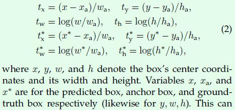
转载于 //www.cnblogs.com/leebxo/p/10784212.html


还没有评论,来说两句吧...